Recent results on the topological fixed point theory of multivalued mappings: a survey

Abstract

In this survey, we present current results from the topological fixed point theory of multivalued mappings which were obtained by ourselves in the last five years (see Andres and Górniewicz in Fixed Point Theory 12(2):255-264, 2011; Topol. Methods Nonlinear Anal. 40:337-358, 2012; Libertas Mathematica 33(1):69-78, 2013; Int. J. Bifurc. Chaos 24(11):1450148, 2014; J. Nonlinear Convex Anal. 16(6):1013-1023, 2015; Int. J. Bifurc. Chaos, 2015, to appear). Some abstract theorems are applied to differential inclusions and multivalued fractals. A part of the deterministic theory is randomized, including the applications to random differential inclusions.

1 Introduction

The topological fixed point theory is a systematically developed discipline whose powerful methods can be effectively applied in many branches of mathematics, mathematical physics and natural science. Its combination with multivalued analysis opens new horizons in exploring more realistic models in mathematical economics, population dynamics and optimal control theory (see e.g. [1, 2]).

It concerns not only the traditional study of optima and equilibria in terms of multivalued dynamical systems and differential inclusions, but also (less traditionally) the fractal structure of invariant sets of discrete dynamical systems corresponding to practically important (possibly robust) stationary collective phenomena, or so.

Plenty of topological fixed point theorems can be found in monographs like [3–10]. Nevertheless, many of them can be still improved or generalised and extended. Furthermore, some results can be also elaborated and adopted for the needs of mentioned applications like multivalued fractals.

In the present survey, we collected such joint results in the field of topological fixed point theory of multivalued mappings obtained by ourselves in the last five years [11–16]. The given fixed point problems concern both deterministic and random processes. The multivalued maps under our consideration, so-called compact absorbing contractions (CAC-maps), contain tendentiously only a small amount of compactness. Besides absolute neighborhood retracts (ANR-spaces), we also consider a more general class of absolute neighborhoods multiretracts (ANMR-spaces) as supporting spaces.

By advanced techniques, based on the Lefschetz-type fixed point theorems and sophisticated degree arguments (fixed point index techniques), we are able to treat not only the sole existence problems, but also to guarantee certain sorts of a weak stability called nonejectivity and essentiality.

The applications deal with deterministic and random differential inclusions, nonejective and essential multivalued fractals. Let us also note that, for multivalued fractals, only single-valued fixed point theorems applied in hyperspaces are needed.

Hence, after some auxiliary preliminaries, ten sections are devoted separately to these problems. For more details and illustrative examples; see [11–16]. Some open problems are formulated as a challenge for a future research.

2 Some auxiliary definitions

In the entire text, all topological spaces are metric and, until Section 6, all single-valued mappings are continuous. Let X be a metric space and let x be a point of X. By $U(x)$, we shall denote the family of all open neighborhoods of x in X.

Let Top₂ be the category of pairs of topological spaces and continuous mappings of such pairs. By a pair $(X, A)$ in Top₂, we understand a space X and its subset A; a pair $(X, \emptyset)$ will be denoted for brevity by X. By a map $f \colon(X, A) \to(Y, B)$, we shall understand a continuous map from X to Y such that $f(A) \subset B$.

We shall use the following notations: if $f\colon(X, A) \to(Y, B)$ is a map of pairs, then by $f_{X} \colon X \to Y$ and $f_{A} \colon A \to B$, we shall understand the respective induced mappings. Let us also denote by $\operatorname {Vect}_{G}$ the category of graded vector spaces over the field of rational numbers $\mathbb{Q}$ and linear maps of degree zero between such spaces. By $H\colon \operatorname {Top}_{2} \to \operatorname {Vect}_{G}$, we shall denote the Čech homology functor with compact carriers and coefficients in $\mathbb{Q}$.

Thus, for any pair $(X, A)$, we have $H(X, A) = \{H_{q} (X, A)\}_{q\geq0}$, a graded vector space in $\operatorname {Vect}_{G}$ and, for any map $f\colon(X, A) \to(Y, B)$, we have the induced linear map $f_{*} = \{f_{*q}\} \colon H(X, A) \to H(Y, B)$, where $f_{*q} \colon H_{q} (X, A) \to H_{q} (Y, B)$ is a linear map from the q-dimensional homology $H_{q} (X, A)$ of the pair $(X, A)$ into the q-dimensional homology $H_{q} (Y, B)$ of the pair $(Y, B)$.

For the properties of H, we recommend [5, 17].

A nonempty space X is called acyclic provided:

• (i) $H_{q}(X) = 0$, for every $q\geq1$, and

• (ii) $H_{0}(X) = \mathbb{Q}$.

Definition 2.1

A map $p \colon\Gamma\to X$ is called a Vietoris map if the following conditions are satisfied:

• (a) p is onto and proper, i.e., $p^{-1}(K)$ is compact for every compact $K\subset X$,

• (b) for every $x \in X$, the set $p^{-1}(x)$ is acyclic.

Theorem 2.2

(Vietoris) (see e.g. [5])

If $p \colon\Gamma\to X$ is a Vietoris map, then the induced linear map $p_{*} \colon H(\Gamma) \stackrel {\sim }{\to} H(X)$ is an isomorphism, i.e. for every $q \geq0$, the linear map $p_{*q} \colon H_{q} (\Gamma) \stackrel {\sim }{\to} H_{q} (X)$ is a linear isomorphism.

For further properties of Vietoris mappings, see e.g. [5, 17].

The following notions will play a crucial role. At first, by $\varphi \colon X \multimap Y$, we shall denote a multivalued map, i.e. a map which assigns to every point $x \in X$ a nonempty set $\varphi(x) \subset Y$. Until Section 6, all multivalued maps will be considered still compact-valued.

A multivalued map $\varphi\colon X\multimap Y$ is called admissible (see [4, 5]) provided there exists a diagram

$$X \,\stackrel {p}{\longleftarrow}\,\Gamma\, \stackrel {q}{\longrightarrow}\, Y $$

in which p is a Vietoris map such that $\varphi(x) = q(p^{-1}(x))$. The pair $(p, q)$ is called a selected pair of φ (written: $(p, q)\subset\varphi$). In what follows, we shall use the following notation:

$$\Gamma \,\stackrel {p}{\Longrightarrow}\, X $$

for Vietoris mappings.

Note that the superposition $\psi\circ\varphi\colon X \multimap Z$ of two admissible maps $\varphi\colon X \multimap Y$ and $\psi\colon Y \multimap Z$ is again an admissible map.

For a map $\varphi\colon X \multimap X$, we shall consider the set $\operatorname {Fix}(\varphi)$ of fixed points φ, i.e.,

$$\operatorname {Fix}(\varphi) := \bigl\{ x \in X \mid x \in\varphi(x)\bigr\} . $$

Denoting, for $\varphi\colon X \multimap Y$, by

$$\varphi^{-1}(B):=\bigl\{ x\in X\mid\varphi(x)\subset B\bigr\} \quad \mbox{and}\quad \varphi_{+}^{-1}(B):=\bigl\{ x\in X\mid\varphi(x)\cap B\neq \emptyset\bigr\} $$

the small and large counter-images of $B\subset Y$, we can still define upper semicontinuous and lower semicontinuous multivalued maps as follows.

Definition 2.3

A mapping $\varphi\colon X \multimap Y$ is said to be upper semicontinuous (u.s.c.) if, for every open $U\subset Y$, the set $\varphi^{-1}(U)$ is open in X or equivalently if, for every closed $U\subset Y$, the set $\varphi_{+}^{-1}(U)$ is closed in X.

A mapping $\varphi\colon X \multimap Y$ is said to be lower semicontinuous (l.s.c.) if, for every closed $U\subset Y$, the set $\varphi^{-1}(U)$ is closed in X or equivalently if, for every open $U\subset Y$, the set $\varphi_{+}^{-1}(U)$ is open in X.

If φ is both u.s.c. and l.s.c., then it is called continuous.

Admissible maps are, in particular, u.s.c. More information as regards admissible mappings will be presented in the next section.

Let us also recall that the space X is an absolute neighborhood retract $(X \in \operatorname {ANR})$, provided there exist an open set U in a normed space E and two maps:

$$r \colon U \to X \quad\mbox{and}\quad s \colon X \to U $$

such that $r \circ s = \mathrm {id}_{X}$; if U is an arbitrary convex set, then X is called an absolute retract ($X\in \operatorname {AR}$).

We shall also use the notion of a multiretraction.

Definition 2.4

([11, 18])

A map $r \colon Y \to X$ is said to be a multiretraction if there exists an admissible map $\varphi\colon X \multimap Y$ such that $r \circ\varphi= \mathrm {id}_{X}$.

Definition 2.5

([11, 18])

A space X is called an absolute neighborhood multiretract $(X \in \operatorname {ANMR})$ if there exist an open set U of a normed space E and a multiretraction $r \colon U \to X$; if U is an arbitrary convex set, then X is an absolute multiretract ($X\in \operatorname {AMR}$).

Evidently, we have

$$\operatorname {ANR}\subset \operatorname {ANMR}, $$

i.e. the class of ANMR-spaces is obviously larger than the one of ANR-spaces (see [11, 18]).

For some nontrivial examples and more details concerning ANMR-spaces, we recommend [18].

Finally, let us recall that a compact space is called an $R_{\delta}$-set provided it is an intersection of a decreasing sequence of compact AR-spaces.

3 Compact absorbing contraction mappings

Let $\varphi\colon X \multimap Y$ be an admissible mapping and $(p,q) \subset\varphi$ be a selected pair of φ.

Using the Vietoris theorem, Theorem 2.2, we are able to define the linear map induced by $(p, q)$ by putting

$$q_{*}\circ p_{*}^{-1}\colon H_{*}(X) \to H_{*}(Y ). $$

We let $\varphi_{*}=\{q_{*}\circ p_{*}^{-1}\mid(p, q) \subset\varphi\}$.

Now, let us consider two admissible mappings $\varphi, \psi\colon X \multimap Y$. We shall say that φ is homotopic to ψ (written: $\varphi\sim\psi$), provided there exists an admissible mapping $\chi\colon X\times[0, 1] \multimap Y$ such that $\chi(x, 0) = \varphi (x)$ and $\chi(x, 1) = \psi(x)$, for every $x \in X$.

We have the following proposition (for its proof, see [5]).

Proposition 3.1

If $\varphi\sim\psi$, then $\varphi_{*}\cap\psi_{*}\neq\emptyset$.

Let $(p_{1}, q_{1}) \subset\varphi$ and $(p_{2}, q_{2})\subset\psi$. We shall say that the above selected pairs are homotopic (written: $(p_{1}, q_{1}) \sim(p_{2}, q_{2})$), provided there exists the following commutative diagram:

where $i_{0}(x) = (x, 0)$, $i_{1}(x) = (x, 1)$, Γ is a given space and f, g are given maps.

Evidently, we have

Proposition 3.2

If $(p_{1}, q_{1})\sim(p_{2}, q_{2})$, then $q_{1*} \circ p_{1*}^{-1}= q_{2*}\circ p_{2*}^{-1}$.

We say that an admissible map $\varphi\colon X \multimap X$ is a Lefschetz map provided, for every selected pair $(p, q) \subset \varphi$, the generalised Lefschetz number $\Lambda(p, q) = \Lambda(q_{*}\circ p_{*}^{-1})$ is well defined and if $\Lambda(p,q)\neq0$, then there exists a point $x\in X$ such that $x\in q(p^{-1}(x))$ (for the definition of the generalised Lefschetz number and more details, see [4, 5, 17]).

For a Lefschetz map $\varphi\colon X\multimap X$, we define the Lefschetz set $\Lambda(\varphi)$ of φ by putting

$$ \Lambda(\varphi):=\bigl\{ \Lambda(p, q) \mid(p, q) \subset\varphi\bigr\} . $$

We have (see [5]):

$$\begin{aligned} &\mbox{If }\varphi\sim\psi, \quad\mbox{then } \Lambda(\varphi) \cap \Lambda (\psi) \neq\emptyset; \end{aligned}$$

(3.1)

$$\begin{aligned} &\mbox{If }(p_{1}, q_{1}) \sim(p_{2}, q_{2}),\quad \mbox{then } \Lambda\bigl((p_{1}, q_{1})\bigr) = \Lambda\bigl((p_{2}, q_{2})\bigr). \end{aligned}$$

(3.2)

Definition 3.3

([4, 5, 17, 19])

An admissible map $\varphi\colon X \multimap X$ is called a compact absorbing contraction ($\varphi\in \operatorname {CAC}(X)$) if there exists an open set $U \subset X$ such that:

• (a) $\varphi(U ) \subset U$,

• (b) the closure ̅ of $\varphi(U )$ is contained in a compact subset of U,

• (c) for every $x \in X$, there exists a natural number $n_{x}$ such that $\varphi^{n_{x}} (x) \subset U$.

We say that $\varphi\colon X \multimap X$ is a locally compact map provided, for every $x \in X$, there exists $V \in U (x)$ such that $\varphi|_{V} \colon V \multimap X$ is a compact map, i.e. ̅ is compact.

We let:

• $\mathrm {K}(X) = \{\varphi\colon X \multimap X \mid\varphi\mbox{ is admissible and compact}\}$.

• $\operatorname {EC}(X) = \{\varphi\colon X \multimap X \mid\varphi\mbox{ is admissible locally compact and there exists a natural}\mbox{ }\mbox{number }n\mbox{ such that the } n\mbox{th iteration }\varphi^{n} \colon X \multimap X\mbox{ of }\varphi\mbox{ is a compact map}\}$.

• $\operatorname {ASC}(X) = \{\varphi\colon X \multimap X \mid\varphi\mbox{ is admissible locally compact, the orbit }O(x) = \bigcup^{\infty}_{n=1} \varphi^{n}(x) \mbox{ is},\mbox{ }\mbox{for every }x \in X,\mbox{ relatively compact and the } \textit{core } C(\varphi) = \bigcap^{\infty}_{n=1} \varphi^{n}(x)\mbox{ is nonempty and}\mbox{ }\mbox{relatively compact}\}$.

• $\operatorname {CA}(X) = \{\varphi\colon X \multimap X \mid\varphi\mbox{ is admissible locally compact and has a } \textit{compact attractor}, \textit{i.e.},\mbox{ }\mbox{then there exists a compact set }A \subset X\mbox{ such that, for every open set }W \subset X\mbox{ containing}\mbox{ }A \mbox{ and for every point }x \in X, \mbox{there is }n_{x}\mbox{ such that }\varphi^{n_{x}} (x) \subset W\}$.

The following hierarchy holds [4, 5]:

$$ \mathrm {K}(X) \subset \operatorname {EC}(X) \subset \operatorname {ASC}(X) \subset \operatorname {CA}(X) \subset \operatorname {CAC}(X). $$

(3.3)

Moreover, each of the above inclusions is proper.

Let $\varphi\in \operatorname {CAC}(X)$ and let U be chosen according to Definition 3.3. Then

$$ \varphi_{U}\colon U \multimap U, \mbox{defined by the formula } \varphi_{U} (x) = \varphi(x),\quad\mbox{for every }x \in U, $$

(3.4)

is a compact admissible map. Recall that if $\psi\colon Y \multimap Y$ is a compact admissible map and $Y \in \operatorname {ANMR}$, then ψ is a Lefschetz map and $\Lambda(\psi) \neq\{ 0\}$ implies that ψ has a fixed point (see [5, 11]).

We prove the following theorem.

Theorem 3.4

Let $\varphi\in \operatorname {CAC}(X)$, where $X \in \operatorname {ANMR}$. Assume further that U is chosen according to Definition  3.3 and $\varphi_{U} \colon U \multimap U$ be a map defined in (3.4). Then φ is a Lefschetz map and $\Lambda(\varphi) \subset\Lambda(\varphi_{U} )$.

Proof

Let $(p, q)$ be a selected pair of φ, i.e., we have a diagram:

$$X \,\stackrel {p}{\Longleftarrow}\,\Gamma\, \stackrel {q}{\longrightarrow}\, X $$

such that $\varphi(x) = q(p^{-1}(x))$, for every $x \in X$. Consider still the following diagram:

$$U \,\stackrel {p_{1}}{\Longleftarrow}\, p^{-1}(U ) \,\stackrel {q_{1}}{\longrightarrow}\, U $$

in which $p_{1}$ and $q_{1}$ are respective restrictions of p and q.

We have also the following diagram:

$$(X, U ) \,\stackrel {\overline {p}}{\Longleftarrow}\,\bigl(\Gamma, p^{-1}(U )\bigr) \, \stackrel {\overline {q}}{\longrightarrow}\,(X, U ) $$

in which $\overline{p}(y) = p(y)$ and $\overline{q}(y) = q(y)$, for every $y \in\Gamma$.

Now, we shall use the following formula proved in [5]. If two Lefschetz numbers from the three numbers $\Lambda(\overline{p},\overline{q})$, $\Lambda(p, q)$ and $\Lambda(p_{1}, q_{1})$ are well defined, then the third one is well defined too, and we have

$$\Lambda(p, q) = \Lambda(\overline{p}, \overline{q}) + \Lambda(p_{1}, q_{1}). $$

Since an open subset of an ANMR-space is an ANMR-space, too, we infer from above that $\Lambda(p_{1}, q_{1})$ is well defined.

Now, since we consider the homology with compact carriers, it follows from Definition 3.3(c) (cf. [5], Proposition (42.2)) that $\Lambda(\overline{p}, \overline{q}) = 0$. Consequently, we see that $\Lambda(p, q)$ is well defined, and $\Lambda(p, q) = \Lambda(p_{1}, q_{1})$. Hence, our theorem follows from the compact case (see [18], Theorem 5.1) by which the proof is completed. □

Corollary 3.5

If $\varphi\in \operatorname {CAC}(X)$ and $X \in \operatorname {ANMR}$, then φ is a Lefschetz map and $\Lambda(\varphi)\neq\{0\}$ implies that φ has a fixed point.

There are several formulations of the Lefschetz fixed point theorem for multivalued mappings (see e.g. [4, 5, 18–22]). Theorem 3.4 seems to be the most general one along the indicated lines. The case of random operators will be considered in Section 7.

4 Fixed point index

Firstly, let us assume that $\varphi\colon X \multimap X$ is a compact admissible map, where $X \in \operatorname {ANR}$.

Let $(p, q) \subset\varphi$ and $V \subset X$ be an open set such that $\{x \in V \mid x \in\varphi(x)\}$ is compact. Then the fixed point index $\operatorname{ind}((p, q), V )$ of the pair $(p, q)$ with respect to V is well defined (see e.g. [4, 5, 23, 24]). Note that $\operatorname{ind}((p, q), V )$ is a rational number in general which is sufficient for our needs. Nevertheless, it can be integer-valued provided still, for instance, X to be an open subset of a normed space, up to a fixed homeomorphism and a fixed retraction, or under suitable additional restrictions imposed on the fibers of p. For more details, see e.g. [4, 5]).

We define the fixed point index of φ as the following set:

$$ \operatorname {Ind}(\varphi, V ) := \bigl\{ \operatorname{ind}\bigl((p, q), V \bigr) \mid(p, q) \subset\varphi\bigr\} . $$

Below, we shall list the important properties of the fixed index which we shall need in the next section.

• (1) (Existence) If $\operatorname{ind}((p, q), V ) \neq0$ ($\operatorname {Ind}(\varphi, V) \neq\{0\}$), then $\operatorname {Fix}(p, q) \cap V \neq\emptyset$, where $\operatorname {Fix}(p,q):=\{x\in X\mid x\in q(p^{-1}(x))\}$.

• (2) (Excision) If $\operatorname {Fix}(\varphi) \cap W \subset V \subset W$ is compact, then

  $$\operatorname{ind}\bigl((p, q), V \bigr) = \operatorname{ind}\bigl((p, q), W \bigr) \quad\bigl(\operatorname {Ind}(\varphi, V ) = \operatorname {Ind}(\varphi, W )\bigr). $$

• (3) (Additivity) If $V_{1}$, $V_{2}$ are open subsets of X such that $V_{1} \cap V_{2} = \emptyset$ and $\operatorname {Fix}(\varphi) \cap V_{1}$, $\operatorname {Fix}(\varphi) \cap V_{2}$ are compact sets, then

  $$\operatorname{ind}\bigl((p, q), V_{1} \cup V_{2}\bigr) = \operatorname{ind}\bigl((p, q), V_{1}\bigr) + \operatorname{ind} \bigl((p, q), V_{2}\bigr). $$

• (4) (Homotopy) If $(p_{1}, q_{1}) \sim(p_{2}, q_{2})$ ($\varphi\sim\psi$), then

  $$\operatorname{ind}\bigl((p_{1}, q_{1}), V \bigr) = \operatorname{ind}\bigl((p_{2}, q_{2}), V \bigr)\quad \bigl(\operatorname {Ind}( \varphi, V ) \cap \operatorname {Ind}(\psi, V ) \neq\emptyset\bigr), $$

  where $(p_{1}, q_{1}) \subset\varphi$ and $(p_{2}, q_{2}) \subset\psi$.

• (5) (Normalization) If $V = X$, then

  $$\operatorname{ind}\bigl((p, q), V \bigr) = \Lambda\bigl((p, q)\bigr) \quad\mbox{and}\quad \operatorname {Ind}(\varphi, V )=\Lambda(\varphi). $$

Now, we shall consider the noncompact case. Assume that $\varphi \colon X \multimap X$ is an admissible compact absorbing contraction and $X \in \operatorname {ANR}$. Assume, furthermore, that V is an open set such that $\{x \in V \mid x \in\varphi(x)\}$ is compact. According to Definition 3.3(a), we select an open set U satisfying all assumptions of Definition 3.3. Evidently, $\operatorname {Fix}(\varphi) \subset U$. Moreover, we see that $\varphi_{U} \colon U \multimap U$ is a compact admissible map, where $\varphi_{U} (x) = \varphi(x)$, for every $x \in U$. Let $(p, q)\subset \varphi$. Then $(p_{U} , q_{U} ) \subset\varphi_{U}$, where $p_{U} \colon p^{-1}(U ) \Rightarrow U$ and $q_{U} \colon p^{-1}(U ) \to U$ are defined as follows: $p_{U} (y) = p(y)$ and $q_{U} (y) = q(y)$, for every $y \in p^{-1}(U )$.

We let:

$$ \operatorname{ind}\bigl((p, q), V \bigr) := \operatorname{ind}\bigl((p_{U} , q_{U} ), V \cap U \bigr) $$

(4.1)

and

$$ \operatorname {Ind}(\varphi, V ) := \bigl\{ \operatorname{ind}\bigl((p, q), V \bigr) \mid(p, q) \subset\varphi\bigr\} . $$

(4.2)

By means of (3), we deduce that the definitions (4.1) and (4.2) do not depend on the choice of U. Thus, all properties (1)-(5) are satisfied.

For more details, we recommend [4, 5, 15, 23, 24].

Open Problem 1

Is it possible to define a fixed point index for CAC-mappings on ANMR-retracts?

5 Ejective fixed points

In this section, we shall assume that all multivalued maps are compact absorbing contractions (CAC-maps).

Definition 5.1

([5, 15, 23, 24])

Let $\varphi\colon X\multimap X$ be a given map and let $x_{0}\in \operatorname {Fix}(\varphi)$.

• (a) We say that $x_{0}$ is ejective relative to $V\in U(x_{0})$ if, for any $x\in\overline{V}\setminus\{x_{0}\}$, there exists an integer $n\geq1$ such that $\varphi^{n}(x)\subset X\setminus\overline{V}$. If there exists $V\in U(x_{0})$ such that $x_{0}$ is ejective relative to V, then $x_{0}$ is called ejective. The set of all ejective fixed points is denoted by $\operatorname {Fix}_{e}(\varphi)$.

• (b) A fixed point $x_{0}\in \operatorname {Fix}(\varphi)$ is called repulsive relative to $V\in U(x_{0})$ if, for any $W\in U(x_{0})$, there exists an integer $n(W)\geq1$ such that $\varphi^{n}(X\setminus W)\subset X\setminus\overline{V}$, for all $n\geq n(W)$. If there exists $V\in U(x_{0})$ such that $x_{0}$ is repulsive relative to V, then $x_{0}$ is called repulsive. The set of all repulsive fixed points is denoted by $\operatorname {Fix}_{r}(\varphi)$.

As an immediate consequence of the above definitions, we have:

$$\operatorname {Fix}_{r}(\varphi)\subset \operatorname {Fix}_{e}(\varphi). $$

The following example shows that the converse is not true even for single-valued mappings.

Example 5.2

Let $f\colon[0,1]\to[0,1]$ be defined by the formula

$$f(x)=2\bigl(-x^{2}+x\bigr). $$

Then $x_{0}=0$ is ejective relative to $V=[0,1/4)$. However, 0 is not a repulsive point because $f(1)=0$.

Remark 5.3

Observe that every ejective fixed point is isolated in the set $\operatorname {Fix}(\varphi)$. Therefore, if $\#\operatorname {Fix}_{e}(\varphi)<\infty$, then $\operatorname {Fix}_{e}(\varphi)$ is open and compact in $\operatorname {Fix}(\varphi)$.

Let $\varphi\colon X\multimap X$ be a CAC-map and let $U\subset X$ be chosen according to Definition 3.3. Then we have a compact admissible map $\varphi_{U}\colon U\to U$ defined by $\varphi_{U}(x)=\varphi(x)$, for every $x\in U$. Observe that, in view of (3.4), we have

$$\begin{aligned} &\operatorname {Fix}(\varphi) = \operatorname {Fix}(\varphi_{U}), \end{aligned}$$

(5.1)

$$\begin{aligned} &\operatorname {Fix}_{e}(\varphi) = \operatorname {Fix}_{e}(\varphi_{U}), \end{aligned}$$

(5.2)

$$\begin{aligned} &\operatorname {Fix}_{r}(\varphi) = \operatorname {Fix}_{r}(\varphi_{U}). \end{aligned}$$

(5.3)

Therefore, all results obtained in [23, 24] can be reformulated for CAC-mappings. Note that the class of compact attraction mappings considered in [23, 24] is involved in the class of CAC-mappings (see (3.3)). Consequently, from (5.1)-(5.3), we can deduce the analogous results for compact admissible mappings on ANR-s, for all classes in (3.3).

For example, we can formulate the following two most important theorems.

Theorem 5.4

Let $X\in \operatorname {ANR}$ and $\varphi\colon X\multimap X$ be a CAC-map. Assume furthermore that $x_{0}$ is a repulsive fixed point of φ with respect to $V\in U(x_{0})$. If there exists $W\in U(x_{0})$ such that:

• (a) $\overline{V}\subset U$,

• (b) the inclusion map $i\colon X\setminus W\to X$ induces the isomorphism

  $$i_{*}\colon H_{*}(X\setminus W)\,\stackrel {\sim }{\longrightarrow}\, H_{*}(X), $$

then $\operatorname {Ind}(\varphi, V)=\{0\}$.

Corollary 5.5

If we assume additionally that $\operatorname {Fix}_{r}(\varphi)$ is a finite set and that ${\Lambda}(\varphi)\neq\{0\}$, then there exists a nonrepulsive fixed point of φ.

Concerning ejective fixed points, we will formulate the following theorem.

Theorem 5.6

Let $X\in \operatorname {ANR}$ and $\varphi\colon X\multimap X$ be a CAC-mapping. Assume that

$$ \varphi\bigl(X\setminus \operatorname {Fix}_{e}(\varphi)\bigr)\subset X \setminus \operatorname {Fix}_{e}(\varphi) \quad\textit{and} \quad\#\operatorname {Fix}_{e}(\varphi)< \infty. $$

(5.4)

Denote by $\varphi'\colon(X\setminus \operatorname {Fix}_{e}(\varphi))\multimap (X\setminus \operatorname {Fix}_{e}(\varphi))$ and $\overline{\varphi}\colon(X, X\setminus \operatorname {Fix}_{e}(\varphi))\multimap (X,X\setminus \operatorname {Fix}_{e}(\varphi))$ the respective maps induced by φ. Then we have:

• (a) φ̅ is a Lefschetz map,

• (b) ${\Lambda}(\overline{\varphi})=\{0\}$ and if ${\Lambda}(\varphi)\neq \{0\}$, then $\varphi'$ has a nonejective fixed point.

Denoting still by $\operatorname {Fix}_{et}(\varphi)\subset \operatorname {Fix}_{e}(\varphi)$ the subset of trivial (obvious) ejective fixed points of φ, we can immediately reformulate Theorem 5.6 in the following form which is suitable for applications, for instance, to functional differential equations.

Theorem 5.7

Let $X\in \operatorname {ANR}$ and $\varphi\colon X\multimap X$ be a CAC-mapping. Assume that

$$ \varphi\bigl(X\setminus \operatorname {Fix}_{et}(\varphi)\bigr)\subset X \setminus \operatorname {Fix}_{et}(\varphi) \quad\textit{and}\quad \#\operatorname {Fix}_{et}(\varphi)< \infty. $$

(5.5)

Denote by $\widetilde{\varphi}\colon(X\setminus \operatorname {Fix}_{et}(\varphi ))\multimap(X\setminus \operatorname {Fix}_{et}(\varphi))$ and $\widehat{\varphi}\colon(X, X\setminus \operatorname {Fix}_{et}(\varphi))\multimap (X,X\setminus \operatorname {Fix}_{et}(\varphi))$ the respective maps induced by φ. Then we have:

• (a) φ̂ is a Lefschetz map,

• (b) ${\Lambda}(\widehat{\varphi})=\{0\}$ and if ${\Lambda }(\varphi )\neq\{0\}$, then φ̃ has either a nontrivial ejective fixed point or a nonejective fixed point.

Let us note that some further results concerning repulsive and ejective fixed points for CA-mappings were presented in [15, 23, 24].

As already pointed out, all the results in [23, 24] as well as those for single-valued maps (see e.g. [25]) can be reformulated for CAC-mappings. The proofs are quite analogous to those presented in the quoted papers.

Open Problem 2

Is it possible to prove some existence results about ejective or repulsive fixed points for compact admissible mappings on ANMR-spaces?

6 Possible application to autonomous functional differential inclusions

Now, we will indicate a possible application of ejective fixed points to differential inclusions (see [15]). Consider the following functional inclusion:

$$ x'(t)\in F_{k,l}\bigl(x(t-1)\bigr), $$

(6.1)

where $F_{k,l}(x)\equiv F_{k,l}(x+\omega)$, $\omega>0$, and

$$F_{k,l}(x):= \textstyle\begin{cases} [-\frac{k}{2}, \frac{k}{2} ], & \mbox{for } x\in \{0,\frac{\omega}{2} \},\\ \frac{k}{2}+l\sin (\frac{2\pi}{\omega}x ), &\mbox{for } x\in (0,\frac{\omega}{2} ),\\ -\frac{k}{2}+l\sin (\frac{2\pi}{\omega}x ), & \mbox{for } x\in (\frac{\omega}{2},\omega ). \end{cases} $$

Observe that, for $k=0$, we have

$$F_{0,l} (x):=l\sin \biggl(\frac{2\pi}{\omega}x(t-1) \biggr), $$

by which (6.1) reduces to the delayed differential equation

$$ x'(t)=l\sin \biggl(\frac{2\pi}{\omega}x(t-1) \biggr), $$

(6.2)

studied in a more general form, e.g. in [26].

It was shown that, besides other things, for suitable values of $l>0$, (6.2) possesses hyperbolic nontrivial periodic solutions oscillating around the unstable equilibria given by $\ldots,-\omega ,0,\omega,\ldots$ , and with transversal heteroclinic connections between them.

For (6.1) with $k>0$, the situation becomes more delicate. On one side, one can readily check that again

$$F_{k,l}(x)>0,\quad \mbox{for } x\in \biggl(0,\frac{\omega}{2} \biggr), \quad\mbox{and}\quad F_{k,l}(x)< 0,\quad \mbox{for } x\in \biggl(\frac{\omega}{2},\omega \biggr). $$

Therefore, for the stationary solution $x_{1}(t)\equiv\omega/2$, there is a negative feedback on the circle $S^{1}$ with a reaction lag, i.e.

$$x(t-1)\in \biggl(0,\frac{\omega}{2} \biggr) \quad\mbox{implies}\quad x'(t)>0, $$

and

$$x(t-1)\in \biggl(\frac{\omega}{2},\omega \biggr) \quad\mbox{implies}\quad x'(t)< 0, $$

while for $x_{2}(t)\equiv0$, the feedback is positive.

On the other hand, the associated Poincaré return operator φ is naturally multivalued.

Since $|F_{k,l}(x)|\leq l+ k/2$ holds, for all $x\in\mathbb{R}$, $k>0$, $l>0$, the locally absolutely continuous solutions $x( \cdot)$ of (6.2) are equi-continuous, because they have uniformly bounded derivatives $x'( \cdot)$ such that $|x'( \cdot)|\leq l+k/2$, for almost all $t\in\mathbb{R}$. Therefore, the bounded domain of the Poincaré return operator φ, associated with (6.2), can be a compact subset X of the Banach space of continuous real functions, on the initial interval $[-1,0]$, endowed with the sup-norm. If X is still a retract of this Banach space, or of its convex subset, then the Poincaré return operator φ is defined on a compact AR-space.

Following and matching the ideas in [4], Chapter III.4, and [26], one might expect that the Poincaré return operator φ, associated with (6.2), can be an admissible mapping which, in view of the above arguments, is compact. Moreover, since φ can be defined on a compact AR-space X, we have immediately that $\#\operatorname {Fix}_{e}(\varphi)<\infty$, and especially that $\Lambda(\varphi)\neq\{0\}$ (see Corollary 3.5).

Hence, in order to apply Theorem 5.7, we could only check in this way condition (5.5), provided all the above arguments are satisfied. Of course, in the case of $\operatorname {Fix}_{et}(\varphi)=\operatorname {Fix}_{e}(\varphi)$, Theorem 5.7 coincides with Theorem 5.6. Anyway, for suitable values of $k\geq0$ and $l>0$, inclusion (6.1) would then possess a nontrivial periodic solution.

7 Multivalued random operators

In order to deal with random operators, random fixed points and random orbits, we need to recall the appropriate definitions and basic results. Unlike in the foregoing sections, multivalued maps are not necessarily compact-valued, but only with nonempty values.

By a measurable space, we shall mean as usual the pair $(\Omega ,\Sigma)$, where a set Ω is equipped with a σ-algebra Σ of subsets. We shall use $\mathbb{B}(X)$ to denote the Borel σ-algebra on X. The symbol $\Sigma\otimes\mathbb{B}(X)$ denotes the smallest σ-algebra on $\Omega\times X$ which contains all the sets $A\times B$, where $A\in\Sigma$ and $B\in \mathbb{B}(X)$.

For $\varphi\colon X\multimap Y$, we can define by means of the small and large counter-images of $B\subset Y$, i.e.

$$\varphi^{-1}(B):=\bigl\{ x\in X\mid\varphi(x)\subset B\bigr\} \quad\mbox{and}\quad \varphi^{-1}_{+}(B):=\bigl\{ x\in X\mid\varphi(x)\cap B\ne \emptyset\bigr\} , $$

(weakly) measurable multivalued maps as follows.

Definition 7.1

Let $(\Omega,\Sigma)$ be a measurable space and Y be a separable metric space. A map $\varphi\colon\Omega\multimap Y$ with closed values is called measurable if $\varphi^{-1}(B)\in\Sigma$, for each open $B\subset Y$, or equivalently, if $\varphi^{-1}_{+}(B)\in \Sigma$, for each closed $B\subset Y$. It is called weakly measurable if $\varphi^{-1}_{+}(B)\in\Sigma$, for each open $B\subset Y$, or equivalently, if $\varphi^{-1}(B)\in\Sigma$, for each closed $B\subset Y$.

It is well known that, for compact-valued maps $\varphi\colon\Omega \multimap Y$, the notions of measurability and weak measurability coincide. Moreover, if φ and ψ are measurable, then so is their Cartesian product $\varphi\times\psi$. For more properties and details, see [4–6].

As an important tool in our investigations, we shall employ a version of the Aumann selection theorem which we state here in the form of lemma (see e.g. [6], Theorem 2.2.14).

Lemma 7.2

If $\varphi\colon\Omega\multimap Y$, where Ω is a complete measure space and Y is a complete separable metric space, is a multivalued map whose graph

$$\Gamma_{\varphi}:=\bigl\{ (\omega,y)\in\Omega\times Y\mid y\in\varphi ( \omega)\bigr\} $$

is measurable, i.e. $\Gamma_{\varphi}\in\Sigma\otimes \mathcal{B} (Y)$, then φ possesses a measurable (single-valued) selection $f\subset\varphi$.

Remark 7.3

If $\varphi\colon\Omega\multimap Y$ is measurable with closed values like in the Kuratowski-Ryll-Nardzewski theorem (see e.g. [4–6]), then its graph $\Gamma_{\varphi}$ is measurable (cf. e.g. [6]), and subsequently φ possesses a measurable selection $f\subset \varphi$.

In the sequel, Ω will be always a complete measure space and X be always a complete separable metric space.

Definition 7.4

([12, 27, 28])

Let $A\subset X$ be a closed subset and $\varphi\colon\Omega\times A\multimap X$ be a multivalued map with closed values. We say that φ is a random operator if it is product-measurable (measurable in the whole), i.e. measurable w.r.t. minimal σ-algebra $\Sigma \otimes\mathcal{B} (X)$, generated by $\Sigma\times\mathcal{B} (X)$, where $\mathcal{B} (X)$ denotes the Borel sets of X. If $\varphi(\omega, \cdot)\colon A \multimap X$ is still u.s.c. (or l.s.c.), then φ is called a random u-operator (or a random l-operator).

Remark 7.5

For the definition of a random operator, it is usually still required φ to be compact-valued (cf. [4, 5]), and $\varphi(\omega, \cdot)\colon A\multimap X$ to be u.s.c. or Hausdorff continuous (cf. [6]), for almost all $\omega\in\Omega$. Since these restrictions are not necessary for us, we omitted them in Definition 7.4.

Definition 7.6

Let $A\subset X$ be a closed subset and $\varphi\colon\Omega\times A\multimap X$ be a random operator. We say that φ has a random fixed point ξ if there exists a measurable mapping $\xi\colon\Omega\to A$ such that

$$\xi(\omega)\in\varphi\bigl(\omega,\xi(\omega)\bigr), \quad\mbox{for every }\omega \in \Omega. $$

We let $\operatorname {Fix}^{ra}(\varphi):=\{\xi\colon\Omega\to A\mid\xi \mbox{ is a random fixed point for }\varphi\}$.

A sequence of measurable maps $\{\xi_{i}\}^{k-1}_{i=0}$, where $\xi _{i}\colon\Omega\to A$, $i=0,\ldots, k-1$, is called a random k-orbit, associated to φ, if

• (i) $\xi_{i+1}(\omega)\in\varphi(\omega, \xi_{i}(\omega))$, $i=0,\ldots, k-2$ and $\xi_{0}(\omega)\in\varphi(\omega, \xi _{k-1}(\omega ))$, for almost all $\omega\in\Omega$,

• (ii) the sequence $\{\xi_{i}\}^{k-1}_{i=0}$ is not formed by going p-times around a shorter subsequence of m consecutive elements, where $mp=k$.

If still

• (iii) $\xi_{i}(\omega)\neq\xi_{j}(\omega)$; $i\neq j$; $i,j=0,\ldots , k-1$, for almost all $\omega\in\Omega$,

then we speak about a random primary k-orbit

One can readily check that the notion of a random 1-orbit coincides with the one of a random fixed point.

The following lemma is crucial in our considerations.

Lemma 7.7

Let X be a separable space, A a closed subset of X and $\varphi \colon\Omega\times X\multimap X$ a measurable map with nonempty closed values. We let $\varphi_{\omega}\colon A\multimap X$, $\varphi_{\omega}(x):=\varphi (\omega,x)$. Assume further that, for every $\omega\in\Omega$, the set $\operatorname {Fix}\varphi_{\omega}:=\{x\in X\mid x\in\varphi_{\omega}(x)\}$ of fixed points of $\varphi_{\omega}$ is nonempty and closed. Then the map $F\colon\Omega\multimap X$, given by $F(\omega)=\operatorname {Fix}\varphi_{\omega}$, has a measurable selection.

Proof

Firstly, we define the function $f\colon\Omega\times A\to[0,\infty)$ by putting

$$f(\omega,x):=\operatorname{dist}\bigl(x,\varphi(\omega,x)\bigr)=\inf\bigl\{ d(x,y) \mid y\in \varphi(\omega,x)\bigr\} . $$

Since φ is measurable, so is f (cf. [4, 5]).

Now, it is obvious that the graph $\Gamma_{F}=\{(\omega,x)\in\Omega\times X\mid x\in F(\omega)\}$ of F is equal to $f^{-1}(0)=\{(\omega,x)\in\Omega\times A\mid f(\omega,x)=0\}$.

Since f is measurable, so is the set $\Gamma_{F}=f^{-1}(0)$, and consequently $F\colon\Omega\multimap X$ is measurable on the graph. By virtue of the Aumann-type selection theorem (see Lemma 7.2), there exists a measurable selection $v\colon\Omega\to X$ of F which completes the proof. □

Note that if φ is a random l-operator, then it is sufficient to assume in Lemma 7.2 only that $\varphi( \cdot,x)$ is measurable, for every $x\in X$.

In order to formulate the generalisation of Lemma 7.7 for random orbits, it will be useful to split Ω in the following way (μ denotes a measure):

$$ \textstyle\begin{cases} \Omega=\Omega_{0}\cup\bigcup_{m|k} \Omega_{m}, \mbox{ where }\mu(\Omega_{0})=0, \mbox{all }\Omega_{m}\mbox{'s are measurable}, \\ \mbox{there are }i_{0},\ldots,i_{l}\mbox{ such that }\mu(\Omega_{i_{j}})>0,\mbox{ for all }i_{j}\mbox{'s}, \\ \mbox{and the least common multiple of }i_{j}\mbox{'s is }k. \end{cases} $$

(7.1)

Defining the multivalued maps

$$\mathbb{O}_{k}\colon\Omega\multimap A^{k},\quad k\in \mathbb {N}\quad\mbox{and}\quad \mathbb{O}_{m}^{k/m} \upharpoonright_{\Omega_{m}}\colon \Omega_{m} \multimap A^{k} $$

by

$$\mathbb{O}_{k}(\omega):= \bigl\{ \{x_{i} \}_{i=0}^{k-1}\in A^{k}\mid\{x_{i}\} _{i=0}^{k-1} \mbox{ is a }k\mbox{-orbit of }\varphi(\omega, \cdot) \bigr\} $$

and

$$\begin{aligned} \mathbb{O}_{m}^{k/m}\upharpoonright_{\Omega_{m}} ( \omega):={}& \biggl\{ \{ x_{i}\} _{i=0}^{k-1}\in A^{k} \Bigm| \{x_{i}\}_{i=0}^{m-1}\mbox{ is an } m\mbox{-orbit of }\varphi (\omega, \cdot)\\ &{}\mbox{and } x_{i+tm}=x_{i},\mbox{ for } t=1,\ldots, \frac{k}{m} \biggr\} , \end{aligned}$$

i.e. $\mathbb{O}_{m}^{k/m}(\omega) \upharpoonright_{\Omega_{m}}$, $\omega\in\Omega_{m}$, is a set of m-orbits repeated $(k/m)$-times, we are ready to give the following crucial statement, whose ‘if-part’ was proved in [27] (the ‘only if-part’ follows directly from the definition of a random k-orbit).

Lemma 7.8

Assume that $\varphi\colon\Omega\times A\multimap X$ is a random operator. Then φ admits a random k-orbit, $k\in \mathbb {N}$, if and only if $\mathbb{O}_{m}(\omega)$ is, under (7.1), nonempty, for all $\omega\in\Omega_{m}$, where $m|k$.

In particular, we can still give the following corollary.

Corollary 7.9

If the set $\mathbb{O}_{k}(\omega)$ of orbits of $\varphi(\omega, \cdot )$ is nonempty, for almost every $\omega\in\Omega$, then φ admits a random k-orbit.

Remark 7.10

Observe that, for $k=1$, Corollary 7.9 implies that the set $\operatorname {Fix}\varphi_{\omega}$ need not be closed like in Lemma 7.7.

8 Lefschetz fixed point theorem for random multivalued mappings

In this section, we will present a version of the Lefschetz fixed point theorem for random operators. Our result can be regarded as a completion of the deterministic Theorem 3.4. For more details, see [12, 13].

Theorem 8.1

Let $\varphi\colon\Omega\times X\multimap X$ be a random u-operator. Assume further that:

• (a) X is a separable ANMR-space,

• (b) $\varphi_{\omega}\colon X\multimap X$, $\varphi_{\omega }(x)=\varphi(\omega, x)$ is a CAC-map, for every $\omega\in\Omega$.

Then:

• (i) $\varphi_{\omega}\colon X\multimap X$ is a Lefschetz map, and

• (ii) if $\Lambda(\varphi_{\omega})\neq\{0\}$, for almost all $\omega\in\Omega$, then $\operatorname {Fix}^{\mathrm {ra}}(\varphi)\neq\emptyset$.

Proof

Using the deterministic version of the Lefschetz fixed point Theorem 3.4, we infer that, for almost all $\omega\in\Omega$, the set $\operatorname {Fix}(\varphi_{\omega})$ is nonempty. Thus, we can apply Lemma 7.7, and get $\operatorname {Fix}^{\mathrm {ra}}(\varphi)=\{\xi\colon\Omega\to X\mid\xi(\omega)\in \varphi (\omega,\xi(\omega)), \mbox{for every }\omega\in\Omega\}\neq\emptyset$. □

As a particular case of Theorem 8.1, we obtain the following random version of the Schauder fixed point theorem.

Corollary 8.2

If X is a separable AMR-space and $\varphi\colon\Omega\times X\multimap X$ is a random map such that, for every $\omega\in\Omega$, the map $\varphi_{\omega}\colon X\multimap X$ is a CAC-map, then $\operatorname {Fix}^{\mathrm {ra}}(\varphi)\neq\emptyset$.

Open Problem 3

Is Theorem 8.1 valid without the assumption that X is a separable space?

Remark 8.3

Random fixed point theorems for condensing maps were investigated e.g. in [29].

9 Topological degree of random operators

In this section, a random topological degree will be defined for a suitable class of random operators.

Let $\mathbb {R}^{n}$, $n\geq1$, be as usually an n-dimensional real Euclidean space, with the inner product $\langle\cdot, \cdot\rangle$ and the induced norm $\| \cdot\|$. A closed (resp. open) ball in $\mathbb {R}^{n}$ with center x and radius $r>0$ is denoted by $B^{n}(x,r)$ (resp. $B^{n}_{0}(x,r)$). Furthermore, put

$$\begin{aligned}& B^{n}(r) =B^{n}(0,r), \qquad B^{n}_{0}(r)=B^{n}_{0}(0,r),\\& S^{n-1}(r)=B^{n}(r)\setminus B^{n}_{0}(r), \qquad\mathbb{P}^{n}=\mathbb {R}^{n}\setminus\{0\}; \end{aligned}$$

$\mathbb{Z}$ stands for the set of all integers.

For any $X\in \operatorname {ANR}$, we let

$$\begin{aligned} J^{\mathrm {ra}}\bigl(\Omega\times B^{n}(r),X\bigr):={}&\bigl\{ F\colon \Omega\times B^{n}(r)\multimap X\mid F\mbox{ is a random }u\mbox{-operator with }R_{\delta}\mbox{-values}\bigr\} . \end{aligned}$$

For any $X\in \operatorname {ANR}$ and any continuous function $f\colon X\to \mathbb {R}^{n}$, we put

$$\begin{aligned} J_{f}^{\mathrm {ra}}\bigl(\Omega\times B^{n}(r), \mathbb {R}^{n}\bigr) :={}&\bigl\{ \varphi\colon\Omega\times B^{n}(r) \multimap \mathbb {R}^{n}\mid\varphi=f\circ F, \\ &{}\mbox{for some }F\in J^{\mathrm {ra}}\bigl(\Omega\times B^{n}(r),X\bigr),\mbox{ and } \varphi\bigl(\Omega\times S^{n-1}(r)\bigr)\subset\mathbb{P}^{n} \bigr\} . \end{aligned}$$

Finally, we define

$$\begin{aligned} CJ^{\mathrm {ra}}\bigl(\Omega\times B^{n}(r),\mathbb {R}^{n}\bigr):={}& \bigcup\bigl\{ J_{f}^{\mathrm {ra}}(\Omega \times B^{n}(r),\mathbb {R}^{n}\mid\\ &{}f\colon X\to \mathbb {R}^{n} \mbox{ is continuous and }X\in \operatorname{ANR}\bigr\} . \end{aligned}$$

The aim of this section is to introduce the notion of a random topological degree for the class $CJ^{\mathrm {ra}}(\Omega\times B^{n}(r),\mathbb {R}^{n})$. Before doing it, we need an appropriate notion of a homotopy in $CJ^{\mathrm {ra}}(\Omega\times B^{n}(r),\mathbb {R}^{n})$.

Definition 9.1

Let $\varphi_{1},\varphi_{2}\in CJ^{\mathrm {ra}}(\Omega\times B^{n}(r),\mathbb {R}^{n})$ be two maps of the form:

$$\begin{aligned}& \varphi_{1} = f_{1}\circ F_{1}, \qquad \Omega\times B^{n}(r) \stackrel{F_{1}}{\multimap } X \stackrel {f_{1}}{\longrightarrow} \mathbb {R}^{n},\\& \varphi_{2} = f_{2}\circ F_{2}, \qquad \Omega\times B^{n}(r) \stackrel{F_{2}}{\multimap } X \stackrel {f_{2}}{\longrightarrow} \mathbb {R}^{n}. \end{aligned}$$

We say that $\varphi_{1}$ and $\varphi_{2}$ are homotopic in $CJ^{\mathrm {ra}}(\Omega\times B^{n}(r),\mathbb {R}^{n})$ if there exists a random u-operator with $R_{\delta}$-values $\chi\colon\Omega\times B^{n}(r)\times[0,1]\multimap X$ and a continuous homotopy $h\colon X\times[0,1]\to \mathbb {R}^{n}$ such that:

• (a) $\chi(\omega,x,0)=F_{1}(\omega,x)$, for every $\omega\in\Omega$ and $x\in B^{n}(r)$,

• (b) $\chi(\omega,x,1)=F_{2}(\omega,x)$, for every $\omega\in\Omega$ and $x\in B^{n}(r)$,

• (c) $h(x,0)=f_{1}(x)$, $h(x,1)=f_{2}(x)$, for every $x\in B^{n}(r)$,

• (d) for every $(\omega,u,t)\in\Omega\times S^{n-1}(r)\times[0,1]$ and $x\in\chi(\omega,u,t)$, we have $h(x,t)\neq0$.

The mapping $H\colon\Omega\times B^{n}(r)\times[0,1]\multimap \mathbb {R}^{n}$ given by $H(\omega,x,t)=h(\chi(\omega,x,t),t)$ is called a homotopy in $CJ^{\mathrm {ra}}(\Omega\times B^{n}(r),\mathbb {R}^{n})$ between $\varphi_{1}$ and $\varphi_{2}$.

Now, observe that if $\varphi\in CJ^{\mathrm {ra}}(\Omega\times B^{n}(r),\mathbb {R}^{n})$, then $\varphi_{\omega}=\varphi(\omega, \cdot)\in CJ^{\mathrm {ra}}(\{\omega \} \times B^{n}(r),\mathbb {R}^{n})$, for every $\omega\in\Omega$, and so the topological degree $\operatorname{Deg}(\varphi_{\omega})$ of $\varphi _{\omega}$ is well defined (see e.g. [4, 5]). Therefore, we are allowed to define the following.

Definition 9.2

We define a multivalued map $D\colon CJ^{\mathrm {ra}}(\Omega\times B^{n}(r),\mathbb {R}^{n})\multimap\mathbb{Z}$ by putting $D(\varphi):=\{\operatorname{Deg}(\varphi_{\omega})\mid\omega\in \Omega\}$. The map D is called the random topological degree of φ on $CJ^{\mathrm {ra}}(\Omega\times B^{n}(r),\mathbb {R}^{n})$.

In what follows, we say that the random topological degree $D(\varphi)$ of φ is different from zero (written: $D(\varphi)\neq0$) if $\operatorname{Deg}(\varphi_{\omega})\neq0$, for every $\omega\in \Omega$.

Below, we collect the most important properties of the random topological degree.

Theorem 9.3

The multivalued map $D\colon CJ^{\mathrm {ra}}(\Omega\times B^{n}(r),\mathbb {R}^{n})\multimap\mathbb{Z}$ defined in Definition  9.2 has the following properties:

• (a) (Existence) If $D(\varphi)\neq0$, then there exists a measurable function $\xi\colon\Omega\to B^{n}(r)$ such that $0\in\varphi(\omega,\xi (\omega))$, for every $\omega\in\Omega$.

• (b) (Excision) If $\varphi\in CJ^{\mathrm {ra}}(\Omega\times B^{n}(r),\mathbb {R}^{n})$ and $\{(\omega,x)\in\Omega\times B^{n}(r)\mid0\in\varphi(\omega,x)\} \subset\Omega\times B_{0}^{n}(\widetilde{r})$, for some $0<\widetilde{r}< r$, then the restriction φ̃ of φ to $\Omega\times B^{n}(\widetilde{r})$ is in $CJ^{\mathrm {ra}}(\Omega\times B^{n}(\widetilde{r}),\mathbb {R}^{n})$ and $D(\varphi)=D(\widetilde{\varphi})$.

• (c) (Factorization) Let $\varphi_{1},\varphi_{2}\in CJ^{\mathrm {ra}}(\Omega\times B^{n}(r),\mathbb {R}^{n})$ be two maps of the form:

  $$\begin{aligned}& \varphi_{1}= f_{1}\circ F_{1}, \qquad \Omega\times B^{n}(r) \stackrel{F_{1}}{\multimap } X \stackrel {f_{1}}{\longrightarrow} \mathbb {R}^{n},\\& \varphi_{2}= f_{2}\circ F_{2}, \qquad \Omega\times B^{n}(r) \stackrel{F_{2}}{\multimap } Y \stackrel {f_{2}}{\longrightarrow} \mathbb {R}^{n}, \end{aligned}$$

  where $X,Y\in \operatorname {ANR}$. If there exists a continuous map $h\colon X\to Y$ such that the diagram

  

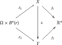
  is commutative, i.e. $F_{2}=h\circ F_{1}$ and $f_{1}=f_{2}\circ h$, then $D(\varphi_{1})=D(\varphi_{2})$.

• (d) (Homotopy) If $\varphi_{1}$ and $\varphi_{2}$ are homotopic in $CJ^{\mathrm {ra}}(\Omega \times B^{n}(r),\mathbb {R}^{n})$, then $D(\varphi_{1})=D(\varphi_{2})$.

Proof

Note that the properties (b)-(d) immediately follow from the respective properties of the function Deg on $CJ^{\mathrm {ra}}(\{\omega\}\times B^{n}(r),\mathbb {R}^{n})$, i.e. for $\varphi_{\omega}\in CJ^{\mathrm {ra}}(\{\omega\}\times B^{n}(r),\mathbb {R}^{n})$ and each $\omega\in\Omega$.

For the proof of (a), observe that for every $\varphi\in CJ^{\mathrm {ra}}(\Omega\times B^{n}(r),\mathbb {R}^{n})$, we can associate the random vector field $\widehat{\varphi}\colon\Omega\times B^{n}(r)\to \mathbb {R}^{n}$ defined as follows:

$$\widehat{\varphi}(\omega,x):=x-\varphi(\omega,x), \quad\mbox{for every }(\omega,x)\in \Omega\times B^{n}(r). $$

If we assume that $D(\varphi)\neq0$ then, for every $\omega\in \Omega$, in view of the existence property for the deterministic topological degree (see e.g. [4], Proposition (8.9.1), p.102), we see that $\operatorname {Fix}(\widehat{\varphi}_{\omega})$ is a nonempty and compact subset of $B^{n}(r)$.

By applying Lemma 7.7, we see that $\xi\in \operatorname {Fix}^{\mathrm {ra}}(\widehat{\varphi})$ which satisfies the following condition: $0\in\varphi(\omega,\xi(\omega))$, for every $\omega\in\Omega$, and the proof is completed. □

It is well known that, from the topological degree theory, one can deduce many topological results like fixed point theorems, theorems on antipodes, theorems on invariant domains, etc.

The same is possible to deduce, under natural suitable assumptions, from the random topological degree. Nevertheless, we restrict our considerations to a random version of the theorem on antipodes.

Theorem 9.4

(Random theorem on antipodes)

Let $\varphi\in CJ^{\mathrm {ra}}(\Omega\times B^{n}(r),\mathbb {R}^{n})$ be a random u-operator such that for every $x\in S^{n-1}(r)$ and for every $\omega\in\Omega$, we have

$$L_{x}\cap\varphi(\omega,x)=\emptyset\quad\textit{or}\quad L_{x}\cap \varphi(\omega,-x)=\emptyset, \quad\textit{where }L_{x}:=\{tx\mid t\geq0\}. $$

Then $D(\varphi)\neq0$.

Proof

For every $\omega\in\Omega$, the map $\varphi_{\omega}\colon B^{n}(r)\to \mathbb {R}^{n}$ satisfies the assumptions of the deterministic Borsuk antipodal theorem (see e.g. [4, 5]). Thus, for every $\omega\in\Omega$, $\operatorname{Deg}(\varphi _{\omega})\neq0$, and our theorem follows from Theorem 9.3(a). □

Finally, we shall sketch the random topological degree theory in Banach spaces. Let E be a separable Banach space. We let:

$$\begin{aligned}& B(r)=\bigl\{ x\in E\mid\Vert x\Vert\leq r\bigr\} ,\\& B_{0}(r)=\bigl\{ x\in E\mid\Vert x\Vert< r\bigr\} ,\\& S(r)=\bigl\{ x\in E\mid\Vert x\Vert= r\bigr\} . \end{aligned}$$

We define $CJ^{\mathrm {ra}}(\Omega\times B(r),E)$ in the same way as $CJ^{\mathrm {ra}}(\Omega\times B(r),\mathbb {R}^{n})$ but we have assumed that, for every $\omega\in\Omega$, the map $\varphi_{\omega}=f\circ F_{\omega}: B(r)\to E$ is compact, i.e. ̅ is a compact subset of E and $\operatorname {Fix}\varphi_{\omega}\subset B_{0}(r)$, for every $\omega\in\Omega$.

As before, with every $\varphi\in CJ^{\mathrm {ra}}(\Omega\times B(r),E)$, we associate the random vector field $\widehat{\varphi}\colon\Omega\times B(r)\multimap E$ by putting: $\widehat{\varphi}(\omega,x)=x-\varphi(\omega,x)$. We let

$$V^{\mathrm {ra}}\bigl(\Omega\times B(r),E\bigr):=\bigl\{ \psi:\Omega\times B(r) \multimap E\mid \psi=\widehat{\varphi}\mbox{ and } \varphi\in CJ^{\mathrm {ra}} \bigl(\Omega\times B(r),E\bigr)\bigr\} . $$

Then we define the map $D\colon V^{\mathrm {ra}}(\Omega\times B(r),E)\multimap Z$ by putting:

$$ D(\psi)=\bigl\{ \operatorname{Deg}(\psi_{\omega})\mid\omega \in\Omega\bigr\} , $$

(9.1)

where $\operatorname{Deg}(\psi_{\omega})$ is the deterministic topological degree of $\psi_{\omega}$ (see e.g. [4], p.104).

The random topological degree defined in (9.1) has all the properties formulated in Theorem 9.3. As a standard consequence of the above random degree theory, we can formulate:

Theorem 9.5

(Random Schauder fixed point theorem)

Let $X\in \operatorname{AR}$ be a closed subset of a separable Banach space E and let $\varphi\colon\Omega\times X\multimap X$ be a random u-operator with $R_{\delta}$-values such that $\varphi_{\omega}\colon X\multimap X$ is compact, for every $\omega\in\Omega$. Then $\operatorname {Fix}^{\mathrm {ra}}(\varphi)\neq\emptyset$.

Note that Theorem 9.5 immediately follows from Corollary 8.2.

Remark 9.6

Let us observe that if $\varphi(\Omega\times S^{n-1}(r))\subset S^{n-1}(\overline{r})$, for some $\overline{r}>0$, then condition (a) in Theorem 9.4 can be replaced by the following one:

$$\varphi(\omega,x)\cap\varphi(\omega,-x)=\emptyset, \quad \mbox{for every } (\omega,x) \in\Omega\times S^{n-1}(r) . $$

We recommend [4, 5] for further formulations of the Borsuk antipodal theorem for multivalued maps in the deterministic case. All the mentioned results have adequate random formulations.

10 Application to random differential inclusions

The second application of our fixed point theorems concerns random differential inclusions. Let $\varphi\colon\Omega\times[0,a]\times \mathbb {R}^{n}\multimap \mathbb {R}^{n}$ be a random u-operator, defined in an analogous way as above on $\Omega\times[0,a]\times \mathbb {R}^{n}$.

Definition 10.1

A random u-operator $\varphi\colon\Omega\times[0,a]\times \mathbb {R}^{n}\multimap \mathbb {R}^{n}$ with convex, compact values is called a random u-Carathéodory map if there exists a map $\mu\colon\Omega\times[0,a]\to[0,\infty)$ such that $\mu(\omega, \cdot)$ is Lebesque integrable, $\mu( \cdot,t)$ is measurable and $\|\varphi(\omega,t,x)\|\leq\mu(\omega,t)(1+\Vert x\Vert)$, for every $\omega\in\Omega$, $t\in[0,a]$ and $x\in \mathbb {R}^{n}$.

Now, for a given random u-Carathéodory map $\varphi\colon\Omega\times[0,a]\times \mathbb {R}^{n}\multimap \mathbb {R}^{n}$ and a measurable map $\xi_{0}\colon\Omega\to \mathbb {R}^{n}$, we shall consider the following Cauchy problem:

$$ (C_{\varphi,\xi_{0}})\quad \textstyle\begin{cases} x'(\omega,t)\in\varphi(\omega,t,x(\omega,t)),\cr x(\omega,0)=\xi_{0}(\omega), \end{cases} $$

where the solution $x\colon\Omega\times[0,a]\to \mathbb {R}^{n}$ is a map such that $x( \cdot,t)$ is measurable, $x(\omega, \cdot)$ is absolutely continuous and the derivative $x'(\omega,t)$ is considered w.r.t. t. In what follows, we shall denote by ${S}(\varphi,\xi_{0})$ the set of all solutions of $(C_{\varphi,\xi_{0}})$.

Theorem 10.2

If $\varphi\colon\Omega\times[0,a]\times \mathbb {R}^{n}\multimap \mathbb {R}^{n}$ is a random u-Carathéodory map, then ${S}(\varphi,\xi_{0})\neq\emptyset$, for any measurable $\xi_{0}\colon\Omega\to \mathbb {R}^{n}$.

For the proof of Theorem 10.2, see [12], Theorem (4.2).

Having a random u-Carathéodory map $\varphi\colon\Omega\times[0,a]\times \mathbb {R}^{n}\multimap \mathbb {R}^{n}$, for every $\omega\in\Omega$ and $y\in \mathbb {R}^{n}$, we can consider the following deterministic Cauchy problem:

$$ (C_{\varphi_{\omega},y})\quad\textstyle\begin{cases} x'(t)\in\varphi_{\omega}(t,x(t)):=\varphi(\omega,t,x(t)),\cr x(0)=y. \end{cases} $$

It is well known (see [4, 5]) that the set $S(\varphi_{\omega},y)$ of all solutions of $(C_{\varphi_{\omega},y})$ is an $R_{\delta}$-set.

We define the map $P\colon\Omega\times \mathbb {R}^{n}\multimap C([0,a],\mathbb {R}^{n})$, by putting:

$$\begin{aligned} P(\omega,y):=S(\varphi_{\omega},y)=\bigl\{ x\in C\bigl([0,a], \mathbb {R}^{n}\bigr)\mid x'(t)\in\varphi_{\omega}\bigl(t,x(t)\bigr)\mbox{ and } x(0)=y\bigr\} . \end{aligned}$$

(10.1)

We can state the following important proposition.

Proposition 10.3

Under the above assumptions, the mapping

$$P\colon\Omega\times \mathbb {R}^{n}\multimap C\bigl([0,a],\mathbb {R}^{n}\bigr) $$

defined in (10.1) is a random u-operator.

Proof

It is well known (see e.g. [4, 5]) that $P(\omega , \cdot)$ is u.s.c. with $R_{\delta}$-values. So, it is sufficient to show that P is measurable. We shall proceed similarly as in the proof of Theorem 10.2 in [12], Theorem (4.2).

Consider the diagram:

in which

$$T(\omega,y):= \biggl\{ u\in L_{1}\bigl([0,a],\mathbb {R}^{n}\bigr) \Bigm| u(t)\in\varphi \biggl(\omega,t,y+\int_{0}^{t} u(\tau)\,d\tau \biggr) \biggr\} $$

but, this time, $L(u)(t)=y+\int_{0}^{t} u(\tau)\,d\tau$. Then $P=L\circ T$ and again it is sufficient to show that T is measurable.

For this, we can proceed quite analogously as in the proof of [12], Theorem (4.2). □

Observe that the measurability of the operator $P\colon\Omega\times \multimap C([0,a],\mathbb {R}^{n})$ says that for any measurable $\xi\colon\Omega\to \mathbb {R}^{n}$, in view of the Kuratowski-Ryll-Nardzewski selection theorem, there exists a measurable selection $\eta\colon\Omega\times \mathbb {R}^{n}\to C([0,a],\mathbb {R}^{n})$ such that $\eta(\omega,x)\subset P(\omega,\xi(\omega))$. Thus, the map $x\colon\Omega\times[0,a]\to \mathbb {R}^{n}$ defined as follows:

$$ x(\omega,t):=\eta(\omega,x) (t) $$

(10.2)

is a solution of $(C_{\varphi,\xi})$.

Note that (10.2) can be reinterpreted in the sense that deterministic solutions define random solutions.

Remark 10.4

Above, we used two times the following fact from measure theory. If $\xi\colon\Omega\to X$ and $\varphi\colon\Omega\times X\multimap Y$ are two measurable maps, then the map $\widehat{\varphi}\colon\Omega\times X\multimap Y$, $\widehat{\varphi}(\omega,x)=\varphi(\omega,\xi(\omega))$ is measurable, too.

In fact, we have the diagram:

$$\Omega \,\stackrel {\widehat{\xi}}{\longrightarrow}\,\Omega\times X \stackrel{\varphi}{ \multimap } Y, $$

where $\widehat{\xi}(\omega)=(\omega,\xi(\omega))$. Then $\hat{\varphi}=\varphi\circ\widehat{\xi}$. Observe that, for any measurable $D\subset\Omega\times X$, the set $\widehat{\xi}^{-1}(D)$ is measurable. Indeed, we can assume without any loss of generality that $D= C\times B$, where $C\subset\Omega$ and $B\subset X$ are measurable. Thus, $\widehat{\xi}^{-1}(D)=C\cap\xi^{-1}(B)$ and ξ̂ has the needed property, because ξ is measurable.

Now, for every measurable $U\subset Y$, we have $\widehat{\varphi}^{-1}(U)=\widehat{\xi}^{-1}(\varphi^{-1}(U))$. Since $\varphi^{-1}(U)$ is measurable, our claim holds true.

Now we shall consider the periodic problem for random differential inclusions. To do it, we shall use the random topological degree.

For a random u-Carathéodory map $\varphi\colon\Omega\times[0,a]\times \mathbb {R}^{n}\multimap \mathbb {R}^{n}$, we shall consider the following periodic problem:

$$ (Q_{\varphi})\quad\textstyle\begin{cases} x'(\omega,t)\in\varphi(\omega,t,x(\omega,t)),\cr x(\omega,0)=x(\omega,a). \end{cases} $$

To study the periodic problem $(Q_{\varphi})$ for such a map φ, we shall follow an approach based on random topological degree theory (for the deterministic case, see e.g. [4, 5]). To do it, consider the random operator $P\colon\Omega\times \mathbb {R}^{n}\multimap C([0,a],\mathbb {R}^{n})$ defined in (10.1) (cf. Proposition 10.3). Moreover, let us consider the evaluation map $e_{a}\colon C([0,a],\mathbb {R}^{n})\to \mathbb {R}^{n}$, $e_{a}(x)=x(a)$. Then the composition

$$ P_{a}:=e_{a}\circ P\colon\Omega\times \mathbb {R}^{n}\multimap \mathbb {R}^{n} $$

(10.3)

is called the random Poincaré operator along the trajectories of $(Q_{\varphi})$.

Assume that $\operatorname {Fix}^{\mathrm {ra}}(P_{a})\neq\emptyset$. This implies that the map: $\widehat{P}\colon\Omega\times \mathbb {R}^{n}\multimap C([0,a],\mathbb {R}^{n})$ given by $\widehat{P}(\omega,y):=\{x\in P(\omega,y)\mid x(0)=x(a)=y\}$ is well defined, i.e. $\widehat{P}(\omega,y)$ is compact and nonempty.

We claim that $\widehat{P}\colon\Omega\times \mathbb {R}^{n}\multimap C([0,a],\mathbb {R}^{n})$ is measurable. Hence, let A be a closed subset of $C([0,a],\mathbb {R}^{n})$. Then we get

$$\widehat{P}^{-1}(A)=P^{-1}\bigl(A\cap\widetilde{e}{}^{-1}(0)\bigr), $$

where $\widetilde{e}\colon C([0,a],\mathbb {R}^{n}) \multimap \mathbb {R}^{n}$, defined by $\widetilde{e}(x)=x(0)-x(a)$, is a continuous map. So P̂ is measurable and, in view of the Kuratowski-Ryll-Nardzewski selection theorem, there exists a measurable selection $\eta\colon\Omega\times \mathbb {R}^{n}\to C([0,a],\mathbb {R}^{n})$ of P̂ which defines a solution of $(Q_{\varphi})$ by putting:

$$x\colon\Omega\times[0,a]\to \mathbb {R}^{n},\quad x(\omega,t):=\eta\bigl(\omega,\xi ( \omega)\bigr) (t), $$

where $\xi\in \operatorname {Fix}^{\mathrm {ra}}(P_{a})$ (cf. Remark 10.4).

Conversely, if we have a solution x of $(Q_{\varphi})$, then the mapping $\xi\colon\Omega\to \mathbb {R}^{n}$, where $\xi(\omega )=x(\omega,0)$, is a fixed point of $P_{a}$. Hence, we have proved:

Proposition 10.5

Problem $(Q_{\varphi})$ has a solution if and only the random Poincaré operator $P_{a}\colon\Omega\times \mathbb {R}^{n}\multimap \mathbb {R}^{n}$ has a random fixed point.

To find a fixed point of $P_{a}$, we associate with $P_{a}$ the random vector field $\widetilde{P}_{a}\colon\Omega\times \mathbb {R}^{n}\multimap \mathbb {R}^{n}$ defined as follows:

$$\widetilde{P}_{a}(\omega,x)=x-P_{a}(\omega,x). $$

Now, we can assume without any loss of generality that $\widetilde{P}_{a}\in CJ^{\mathrm {ra}}(\Omega\times B^{n},\mathbb {R}^{n})$; if not, then $O\in\widetilde{P}_{a}(\omega,x)$, for some $\Vert x\Vert= r$ and every $\omega\in\Omega$, and so $P_{a}$ has a fixed point or, equivalently, our problem $(Q_{\varphi})$ has a solution.

Proposition 10.5 can be still improved in the following way.

Proposition 10.6

Assume that $\widetilde{P}_{a}\in CJ^{\mathrm {ra}}(\Omega\times B^{n}(r),\mathbb {R}^{n})$, for some $r>0$. If $D(\widetilde{P}_{a})\neq0$, then problem $(Q_{\varphi})$ has a solution.

In order to show that $D(\widetilde{P}_{a})\neq0$, we shall adopt to the random case the guiding potential method introduced by Liapunov and subsequently developed by Krasnosel’skiĭ and others (see e.g. [4, 5, 12], and the references therein).

Definition 10.7

A map $V\colon\Omega\times \mathbb {R}^{n}\to \mathbb {R}$ is called a random potential if the following two conditions are satisfied:

• (a) $V( \cdot,x)$ is measurable, for every $x\in \mathbb {R}$,

• (b) $V(\omega, \cdot)$ is a $C^{1}$-map, for every $\omega \in \Omega$.

If $V\colon\Omega\times \mathbb {R}^{n}\to \mathbb {R}$ is a random potential, then we define a random vector field $\partial V\colon\Omega\times \mathbb {R}^{n}\to \mathbb {R}^{n}$ as follows:

$$\partial V(\omega, x):= \biggl(\frac{\partial V}{\partial x_{1}}(\omega ,x),\ldots, \frac{\partial V}{\partial x_{n}}(\omega,x) \biggr), $$

for every $(\omega,x)\in\Omega\times \mathbb {R}^{n}$.

Definition 10.8

Let $V\colon\Omega\times \mathbb {R}^{n}\to \mathbb {R}$ be a random potential. If, for some $r_{0}>r$, V satisfies the following condition:

$$0\notin\partial V\bigl(\Omega\times S^{n-1}(r)\bigr), \quad\mbox{for every } r\geq r_{0}, $$

then V is called a random direct potential.

Let $V\colon\Omega\times \mathbb {R}^{n}\to \mathbb {R}$ be a random direct potential. Observe that $\partial V\in CJ^{\mathrm {ra}}(\Omega\times B^{n}(r),\mathbb {R}^{n})$, for every $r\geq r_{0}$.

So, by Theorem 9.3, $D(\partial V)$ is well defined and, in view of the homotopy property Theorem 9.3(d), it is independent of r. Hence, it makes sense to define the index $I(V)$ of the random direct potential V, by putting $I(V)=D(\partial V)$, where $\operatorname{Deg}(\partial V)$ in Definition 9.2 is considered for $\partial V\in C J^{\mathrm {ra}}(\{\omega\}\times B^{n}(r),\mathbb {R}^{n})$ with $r\geq r_{0}$ and fixed $\omega\in\Omega$.

Some cases of random direct potentials with nonzero index can be found similarly as for deterministic potentials. We restrict our considerations to the following proposition (cf. [4, 12]).

Proposition 10.9

If $V\colon\Omega\times \mathbb {R}^{n}\to \mathbb {R}$ is a random direct potential satisfying

$$\lim_{\Vert x\Vert\to\infty} V(\omega,x)=\infty, \quad\textit{for every }\omega\in \Omega, $$

then $I(V)=\{1\}$.

Proposition 10.9 follows immediately from the deterministic case.

Definition 10.10

Let $\varphi\colon\Omega\times[0,a]\times \mathbb {R}^{n}\multimap \mathbb {R}^{n}$ be a random u-Carathéodory operator and let $V\colon\Omega\times \mathbb {R}^{n}\times \mathbb {R}$ be a random direct potential. We say that V is a random guiding function for φ if the following condition is satisfied:

$$\begin{aligned} &\exists r_{0}>0 \forall(\omega,t,x)\in\Omega\times[0,a] \times \mathbb {R}^{n} \mbox{ with }\|x\|\geq r_{0} \exists y\in \varphi(\omega,t,x): \\ &\bigl\langle y, \partial V(\omega,x)\bigr\rangle \leq0 \mbox{ or } \bigl\langle y, \partial V(\omega,x)\bigr\rangle \geq0 . \end{aligned}$$

(10.4)

Now, we are ready to state the main result of this section.

Theorem 10.11

If $\varphi\colon\Omega\times[0,a]\times \mathbb {R}^{n}\multimap \mathbb {R}^{n}$ is a random u-Carathéodory operator which possesses a random guiding function $V\colon\Omega\times \mathbb {R}^{n}\to \mathbb {R}$ such that $I(V)\neq0$ (cf. e.g. Proposition  10.9), then problem $(Q_{\varphi})$ has a solution.

Sketch of the proof

To prove Theorem 10.11, we need a random version of Lemma 4.5 in [30]. This can be done by making only technical changes in the mentioned lemma. Then the proof of Theorem 10.11 is quite analogous to the proof of Theorem 4.4 in [30]. Instead of the deterministic topological degree, we use here the random topological degree presented in Section 9. □

Remark 10.12

For a nonsmooth (e.g. locally Lipschitz) guiding function V, the analogies of Theorem 10.11 can be given by means of the deterministic theorems. For details see [4], Chapter III.8, [5], Section 72.

Example 10.13

For $V(\omega,x)\equiv V(x):=\frac{\|x\|^{2}}{2}$, we have $V\colon \mathbb {R}^{n}\to \mathbb {R}$, $\partial V(x)=x$, $\|\partial V(S^{n-1}(r))\|=r\geq r_{0}>0$ and $\lim_{\|x\|\to\infty}= \infty\Rightarrow I(V)=\{1\}$. Thus, problem $(Q_{\varphi})$ possesses, according to Theorem 10.11, a random solution, provided $\langle\varphi(\omega,t,x), x\rangle\leq0$ or $\langle\varphi (\omega,t,x), x\rangle\geq0$, for all $\omega\in\Omega$, $t\in[0,a]$ and $\|x\|\geq r_{0}>0$, where $r_{0}$ is a suitable constant.

Finally, we recommend [12] for further information concerning random differential inclusions. Note that the deterministic case is presented in [5], Chapter VI (see also [4], Chapter III.8).

Remark 10.14

For scalar ($n=1$) random inclusions, it was shown in [28] that the existence of a pure subharmonic solution $x_{m}$, where $m>1$, implies the coexistence of subharmonic solutions of all orders $k\in \mathbb {N}$, i.e. $x_{k}(\omega,0)\equiv x_{k}(\omega,ka)$, for every $k\in \mathbb {N}$.

11 Nonejectivity and its application to multivalued fractals

In the last two sections, fixed point theorems for single-valued maps will be applied for obtaining multivalued fractals, i.e. fixed points of special operators induced in hyperspaces or, equivalently, compact subsets of the original spaces which are invariant w.r.t. these multivalued operators. We will deal separately with (strictly) nonejective fixed points (cf. [14]) and essential fixed points (cf. [16]).

Firstly, we recall some related notions. As in the first five sections, all topological spaces are metric, all single-valued mappings are continuous and all multivalued mappings are compact-valued.

By the Hilbert cube, we understand the subset of the Hilbert space $\ell_{2}$ consisting of all sequences $\{x_{k}\}$ with $0\leq x_{k}\leq1/k$, $k=1,2,\ldots$ . It is well known that the Hilbert cube is a compact and convex subset of the $\ell_{2}$-space.

Observe that the Hilbert cube is homeomorphic to the product space of any countable infinity of closed bounded positive length intervals. In particular, it is homeomorphic to the countable product $\prod_{n=1}^{\infty}[0,1]^{n}=[0,1]^{\aleph_{0}}$. Obviously, it has the countably infinite dimension.

It will be also convenient to recall some facts about hyperspaces. If $(X,d)$ is a metric space, then by the associated hyperspace $(K(X),d_{H})$, we mean here the family $K(X):=\{A\subset X \mid A \mbox{ is nonempty and compact}\}$ of compact subsets of X, endowed with the Hausdorff metric $d_{H}$, i.e.

$$d_{H}(A,B):=\max \Bigl\{ \sup_{a\in A} \Bigl(\inf _{b\in B} d(a,b) \Bigr), \sup_{b\in B} \Bigl(\inf _{a\in A} d(a,b) \Bigr) \Bigr\} . $$

It is well known that if X is compact, resp. complete, then so is $K(X)$ (see e.g. [6]). For another important implication, let us recall that X is locally continuum-connected if, for every neighborhood U of each point $x\in X$, there is a neighborhood $V\subset U$ of x such that each point of V can be connected with x by a subcontinuum of U. The following lemma will play an important role in applications (see [31, 32]).

Lemma 11.1

If X is locally continuum-connected, then $K(X)\in \operatorname {ANR}$ and if X is locally continuum-connected and connected, then $K(X)\in \operatorname {AR}$.

If X is locally compact, locally connected and connected, then $K(X)$ is a locally compact AR-space. If X is a nondegenerate Peano’s continuum (i.e. compact, locally connected and connected), then $K(X)$ is up to a homeomorphism, the Hilbert cube, i.e. a special case of a compact AR-space. In particular, if X is a compact AR-space, then the same is true for $K(X)$.

Thus, in view of Lemma 11.1, the Hilbert cube as well as its homeomorphic or retract images are typical examples of compact AR-spaces.

Since by a multivalued map $\varphi\colon X \multimap Y$, we mean here again the one with nonempty, compact values, it will be convenient to use the notation $\varphi\colon X \to K(Y)$.

We say that the mapping $\varphi\colon X \to K(Y)$ is Hausdorff continuous if it is continuous w.r.t. the metric d in X and the Hausdorff metric $d_{H}$ in $K(X)$.

It is well known (see [4–6]) that if $\varphi\colon X \to K(Y)$ is Hausdorff continuous if and only if it is continuous in the sense of Definition 2.3. Furthermore, if $A\subset X$ is a compact subset, then $\varphi(A):=\bigcup_{x\in A} \varphi(x) \subset Y$ is a compact subset of Y, i.e. $\varphi(A)\in K(Y)$. If $\varphi\colon X \to K(Y)$ and $\psi\colon X \to K(Y)$ are continuous, then the same is true for their union $\varphi\cup\psi\colon X \to K(Y)$, where $(\varphi\cup\psi)(x):=\varphi(x)\cup\psi(x)$, for every $x\in X$.

The following implication, which we state here in the form of a lemma, was proved in [33] (cf. [4], Appendix A3).

Lemma 11.2

If $\varphi\colon X\to K(X)$ is continuous and compact in $(X,d)$, then the induced (single-valued) hypermap $\varphi^{*}\colon K(X)\to K(X)$, where $\varphi^{*}(A):=\bigcup_{x\in A} \varphi(x)$, for every $x\in A$, is continuous (in the single-valued setting w.r.t. the Hausdorff metric) and compact in $(K(X),d_{H})$.

Definition 11.3

([34, 35])

We say that a fixed point $x_{0}\in \operatorname {Fix}(f)$ of $f\colon X\to X$ is ejective in the sense of Browder w.r.t. $V\in U(x_{0})$, where $U(x_{0})$ stands for the family of all open neighborhoods of $x_{0}$, if for every $x\in V\setminus\{x_{0}\}$, there exists an integer $n=n(x_{0})\geq1$ such that

$$f^{n}(x)=f\underbrace{\circ\cdots\circ}_{(n-1)\mbox{-}\mathrm{times}} f(x) \in X \setminus V. $$

If there exists $V\in U(x_{0})$ such that $x_{0}$ is ejective in the sense of Browder w.r.t. V, then $x_{0}$ is called ejective in the sense of Browder (briefly, b-ejective). The set of all b-ejective fixed points of f will be denoted by $\operatorname {Fix}_{be}(f)$. If $x_{0}\in \operatorname {Fix}(f)\setminus \operatorname {Fix}_{be}(f)$, then $x_{0}$ is called b-nonejective.

Remark 11.4

Observe that Definition 5.1(a) differs from the above original definition due to Browder [34, 35] in V̅ replaced everywhere by V which we distinguished in Definition 11.3 by the prefix ‘b’.

Definition 11.5

We say that a space X has the nonejective fixed point property ($X\in \operatorname {NEFPP}$) if, for every continuous mapping $f\colon X \to X$, there exists $x_{0}\in \operatorname {Fix}(f)$ such that $x_{0}$ is b-nonejective, i.e. $x_{0}\in \operatorname {Fix}(f)\setminus \operatorname {Fix}_{be}(f)$.

Browder proved the following nonejective fixed point theorem (see [34, 35]).

Theorem 11.6

An infinite-dimensional convex, compact subset of a Banach space has the NEFP-property.

Corollary 11.7

The Hilbert cube has the NEFP-property.

Remark 11.8

Because of finite-dimensional counter-examples (see e.g. [14]), we know that an arbitrary compact AR-space has not the NEFP-property. On the other hand, the set X in Theorem 11.6 can be either noncompact, provided e.g. f is a compact mapping, or finite-dimensional (see again e.g. [14]).

Theorem 11.6 can be generalised in two directions. The first generalisation concerns the preservation of some fixed point properties under a radial retraction.

Definition 11.9

We say that the retraction $r\colon X\to A$ is radial in the point $x_{0}\in A$ if there exist an open neighborhood W of $x_{0}$ in X such that for every $x\in W\setminus A$, we have $r(x)\neq x_{0}$, i.e. $x_{0}\notin r(W\setminus A)$.

Remark 11.10

Observe that if $\operatorname {int}_{X}(A)\neq\emptyset$, then any retraction $r\colon X\to A$ is radial in each point $x\in \operatorname {int}_{X}A$.

Hence, let $g\colon A\to A$ be a continuous mapping. Let us associate with g the mapping $f\colon X\to X$ defined by the formula $f:=i\circ g\circ r$, where $r\colon X\to A$ is a retraction and $i\colon A\to X$ is the inclusion map. In other words, we have the commutative diagram:

One can easily check that the following relationships between f and g hold:

• (i) $f^{n}=f\underbrace{\circ\cdots\circ}_{(n-1)\mbox{-}\mathrm{times}} f = i\circ g^{n}\circ r$, for every integer $n\geq1$,

• (ii) $\operatorname {Fix}(f)=\operatorname {Fix}(g)$,

• (iii) $\operatorname {Fix}_{be}(f)\subset \operatorname {Fix}_{be}(g)$.

Because of (iii), we will prove at first the following proposition.

Proposition 11.11

If $x_{0}\in \operatorname {Fix}_{be}(g)$ and the retraction $r\colon X\to A$ is radial in $x_{0}$, then $x_{0}\in \operatorname {Fix}_{be}(f)$.

Proof

Since r is radial in $x_{0}\in \operatorname {Fix}_{be}(g)$, there is an open neighborhood W of $x_{0}$ in X such that $x_{0}\notin r( W\setminus A)$.

From the ejectivity of $x_{0}$ for g, we get an open neighborhood U of $x_{0}$ in A such that, for every $x\in U\setminus\{x_{0}\}$, there is $n=n(x)$ such that $g(x)\in A\setminus U$.

Letting $V:=W\cap r^{-1}(U)$, we have $x_{0}\in V$, where V is an open neighborhood of $x_{0}$ in X. Consequently, for any $x\in V\setminus\{x_{0}\}$, we see that $f(x)=g(r(x))\neq x_{0}$.

Taking $n=n(r(x))$, we obtain (cf. (i))

$$f^{n}(x)=\bigl(i\circ g^{n}\circ r\bigr) (x)=i\bigl( g^{n}\bigl( r(x)\bigr)\bigr) = g^{n}\bigl(r(x)\bigr)\in A \setminus U \subset X\setminus r^{-1}(U) \subset X\setminus V, $$

i.e. $x_{0}\in \operatorname {Fix}_{be}(f)$, as claimed. □

As a direct consequence of Proposition 11.11 and the inclusion (iii), we can give the following corollary.

Corollary 11.12

If the retraction $r\colon X\to A$ is radial in every ejective fixed point $x\in \operatorname {Fix}_{be}(g)$, then $\operatorname {Fix}_{be}(f)=\operatorname {Fix}_{be}(g)$.

In view of Remark 11.10, we have still the following immediate consequence of Proposition 11.11.

Corollary 11.13

If $\operatorname {Fix}_{be}(g)\subset\operatorname{int}_{X} A\neq\emptyset$, then $\operatorname {Fix}_{be}(f)=\operatorname {Fix}_{be}(g)$.

In the following proposition, we formulate sufficient conditions in order the nonejective fixed points in Theorem 11.6, resp. Corollary 11.7, to be preserved under a radial retraction.

Proposition 11.14

If A is a retract of an infinite-dimensional, convex, compact subset X of a Banach space and $g\colon A\to A$ is a continuous mapping such that $\operatorname {Fix}_{be}(g)\subset\operatorname{int}_{X} A\neq\emptyset$, then g has a nonejective fixed point. The same is true if, in particular, A is an infinite-dimensional retract of the Hilbert cube $[0,1]^{\aleph_{0}}$ and $\operatorname {Fix}_{be}(g)\subset\operatorname{int}_{[0,1]^{\aleph_{0}}} A$.

Proof

According to Theorem 11.6, $f:=i\circ g\circ r\colon X\to X$ defined as above, admits a nonejective fixed point $x_{0}\in \operatorname {Fix}(f) \setminus \operatorname {Fix}_{be}(f)$. Furthermore, in view of (ii), we have $\operatorname {Fix}(f)=\operatorname {Fix}(g)$ and, in view of Corollary 11.13, $\operatorname {Fix}_{be}(f)=\operatorname {Fix}_{be}(g)$. Thus, we can conclude that $x_{0}$ must be a nonejective fixed point of g, i.e. $x_{0}\in \operatorname {Fix}(g) \setminus \operatorname {Fix}_{be}(g)$.

If A is, in particular, an infinite-dimensional retract of $[0,1]^{\aleph_{0}}$ then, in view of (ii), we have $\operatorname {Fix}(f)=\operatorname {Fix}(g)$ and, in view of Corollary 11.13, $\operatorname {Fix}_{be}(f)=\operatorname {Fix}_{be}(g)$. Therefore, since $[0,1]^{\aleph_{0}}\in\operatorname{NEFPP}$ (cf. Corollary 11.7), the same conclusion holds. □

Remark 11.15

Observe that the image $r(X)$ of an open retraction $r\colon X\to r(X)$ of the infinite-dimensional space X need not be infinite-dimensional (e.g. the projection $\Pi\colon[0,1]^{\aleph_{0}}\to[0,1]$) and that the infinite-dimensional retraction $r\colon X\to r(X)$, i.e. $\dim r(X)=\infty$, need not be open (e.g. the deformation $d\colon[0,1]^{\aleph_{0}} \to [0,1/2]^{\aleph_{0}}$, where $d|_{[0,1/2]^{\aleph_{0}}}=\mathrm {id}|_{[0,1/2]^{\aleph_{0}}}$, $d|_{[0,1]^{\aleph_{0}}\setminus[0,1/2]^{\aleph_{0}}}\colon$ $[0,1]^{\aleph_{0}}\setminus[0,1/2]^{\aleph_{0}}\to\partial [0,1/2]^{\aleph_{0}}$, where ∂ denotes the boundary of $[0,1/2]^{\aleph_{0}}$). Moreover, since a linear retraction is a continuous surjection, according to the well known Banach-Schauder theorem, it is an open mapping which can drop the infinite dimension to a finite dimension. Therefore, even a general linear retraction is, without an additional restriction, insufficient for preserving the NEFP-property.

In order to avoid this handicap, we should assume that a linear r is still one-to-one. This namely means that such an r is exactly an isomorphism which preserves a finite dimension. Then r is, however, much more than a linear homeomorphism, and there is no need to have another proposition but Proposition 11.16 below.

The second proposition verifies, in particular, the nonejectivity as a topological property, i.e. its invariance under a homeomorphism. For its proof see [14], Proposition 3.

Proposition 11.16

If $x_{0}\in \operatorname {Fix}(f)\setminus \operatorname {Fix}_{be}(f)$ is a nonejective fixed point of a continuous map $f\colon X \to X$, then $h(x_{0})\in \operatorname {Fix}(g)\setminus \operatorname {Fix}_{be}(g)$ is also a nonejective fixed point of a map $g\circ h=h\circ f\colon h(X)\to h(X)$, where $h\colon X \to h(X)$ is a homeomorphism and $h(X)$ is a homeomorphic image of X.

Hence, combining Propositions 11.14 and 11.16, we can immediately formulate a generalisation of Theorem 11.6 as follows.

Theorem 11.17

Let A be, up to a homeomorphism, a retract image of an infinite-dimensional, convex, compact subset X of a Banach space and $g\colon A \to A$ be a continuous mapping such that

$$\operatorname {Fix}_{be}(h_{1}\circ g)\subset\mathop{\operatorname{int}}\limits_{h_{2}(X)} h_{1}(A)\neq \emptyset, $$

where $h_{1}$, $h_{2}$ are respective homeomorphisms. Then g admits a nonejective fixed point, i.e. $[\operatorname {Fix}(g)\setminus \operatorname {Fix}_{be}(g)]\neq\emptyset$. The same is true if, in particular, $h_{1}(A)$ is an infinite-dimensional retract of the Hilbert cube $h_{2}([0,1]^{\aleph_{0}})$ and

$$ \operatorname {Fix}_{be}(h_{1}\circ g)\subset \mathop{\operatorname{int}}\limits_{h_{2}([0,1]^{\aleph _{0}})} h_{1}(A). $$

(11.1)

In view of Lemma 11.1, the following corollary (for $h_{1}=h_{2}=h^{-1}\colon$ $h(A)\to A$) of Theorem 11.17, which is at the same time also a corollary of Proposition 11.16, will be sufficient for applications to the theory of fractals.

Corollary 11.18

A homeomorphic image of an infinite-dimensional convex, compact subset of a Banach space has the NEFP-property. In particular (cf. Corollary  11.7), a homeomorphic image of the Hilbert cube has the NEFP-property.

Corollary 11.18, jointly with Lemma 11.1, will be now applied to multivalued fractals, considered as nonejective fixed points of the induced special operators (called the Hutchinson-Barnsley operators) in the hyperspace $(K(X),d_{H})$, where X is a Peano’s continuum.

Hence, let $X=(X,d)$ be a Peano’s continuum, i.e. compact, locally connected and connected metric space and $\{\varphi_{i}\colon X \to K(X); i=1,\ldots,m\}$ be a system of multivalued continuous maps with compact values.

According to Lemma 11.1, the hyperspace $(K(X),d_{H})$ is, up to a homeomorphism, the Hilbert cube. Furthermore, the induced (single-valued) hypermaps $\varphi_{i}^{*}\colon K(X) \to K(X)$, $i=1,\ldots,n$, are according to Lemma 11.2 continuous as well as their induced union

$$F^{*}:= \Biggl( \bigcup_{i=1}^{m} \varphi_{i}^{*} \Biggr)\colon K(X)\to K(X), $$

called the Hutchinson-Barnsley operator (see [33], [4], Appendix A.3).

Hence, applying Corollary 11.18, there exists a nonejective fixed point $A_{0}\in K(X)$ of $F^{*}$, i.e. $F^{*}(A_{0})=A_{0}$, which can be immediately reformulated in the form of a theorem as follows.

Theorem 11.19

Let $(X,d)$ be a compact, locally connected and connected metric space and $\{\varphi_{i}\colon X \to K(X); i=1,\ldots,m\}$ be a system of continuous multivalued maps with compact values. Then there exists a compact subset $A_{0}\subset X$ which is positively invariant and nonejective w.r.t. the Hutchinson-Barnsley mapping

$$F:= \bigcup_{i=1}^{m} \varphi_{i} \colon X\to K(X),\quad \textit{i.e. } F(A_{0}):= \bigcup_{x\in A_{0}} \bigcup_{i=1}^{m} \varphi_{i} (x)=A_{0}, $$

and such that (nonejectivity):

$$\begin{aligned} &\forall\varepsilon>0 \exists A_{1}\in K(X), A_{1}\neq A_{0}, \textit{ and } d_{H}(A_{0},A_{1})< \varepsilon\colon \\ &F^{n}(A_{1})=F\underbrace{\circ\cdots \circ}_{(n-1)\mbox{-}\mathrm{times}} F(A_{1}) = \Biggl[ \bigcup _{x\in A_{0}} \bigcup_{i=1}^{m} \varphi_{i} (x) \Biggr]^{n} \\ &\hphantom{F^{n}(A_{1})}\subset\bigl\{ A\in K(X) \mid d_{H}(A_{0},A)< \varepsilon \bigr\} , \quad\textit{for all } n\geq1. \end{aligned}$$

We recommend [14] for some examples and further remarks.

12 Essentiality and its application to multivalued fractals

As in the foregoing section, all topological spaces are metric, all single-valued mappings are continuous and all multivalued mappings are compact-valued.

Let us choose the following notations:

$$C(X,X):=\{ f\colon X\to X\mid f\mbox{ is continuous and compact}\} $$

and

$$C_{0}(X,X):=\bigl\{ f\in C(X,X)\mid\dim \operatorname {Fix}(f)=0\bigr\} , $$

where $\dim(\cdot)$ stands for the topological (Lebesgue covering) dimension.

We endow these classes with the metric ρ given by

$$\rho(f,g):=\sup_{x\in X} d\bigl(f(x),g(x)\bigr). $$

Obviously, for a compact X, we can take

$$\rho(f,g):=\max_{x\in X} d\bigl(f(x),g(x)\bigr). $$

We say that two mappings $f,g\colon X\to X$ are δ-near if $\rho(f,g)<\delta$. Furthermore, the homotopy $h\colon X\times[0,1]\to X$ is said to be an ε-homotopy ($\varepsilon>0$) if, for every $x\in X$, the set $\{h(x,t)\mid t\in[0,1]\}$ has a diameter smaller than ε; if h is an ε-homotopy linking f and g, then we say that f and g are ε-homotopic.

The following statement was proved in [36].

Lemma 12.1

Let $X\in \operatorname {ANR}$ be compact and let $\varepsilon>0$ be a given number. Then there exists $\delta>0$ such that any two δ-near maps $f,g\colon X\to X$ are ε-homotopic.

Following the standard definition of an essential fixed point in [37], we will give a slight modification of it for an isolated fixed point.

Definition 12.2

Let $x_{0}$ be an isolated fixed point of $f\colon X\to X$. We say that $x_{0}\in X$ is an essential fixed point of f if, for every open ε-neighborhood $\mathcal{U}$ of $x_{0}$, there exists $\delta=\delta(\varepsilon)>0$ such that any map $g\colon X\to X$ which is δ-near to f has a fixed point in $\mathcal{U}$.

Let us still denote

$$\operatorname {Ess}(f):=\bigl\{ x\in \operatorname {Fix}(f)\mid x\mbox{ is essential}\bigr\} $$

the set of essential fixed points of f.

By an open (ε-)neighborhood $\mathcal{U}$ of a point $x_{0}\in X$, we understand as usually the set $\mathcal{U}:=\{ x\in X\mid d(x,x_{0})<\delta\}$, for some $\varepsilon>0$. Analogously, by an open (δ-)neighborhood $\mathcal{U}$ of a function $f\in C(X,X)$, we will understand the set $\mathcal{U}:=\{ g\in C(X,X)\mid\rho (f,g)<\delta\}$, for some $\delta>0$.

Let us denote by $\mathcal{U}(x_{0})$ the set of all open neighborhoods of $x_{0}\in X$ and by $\mathcal{U}(f)$ the set of all open neighborhoods of $f\in C(X,X)$.

In view of the above notation, Definition 12.2 can be easily reformulated as follows: for every $\mathcal{U}\in\mathcal{U}(x_{0})$, there exists $V\in \mathcal{U}(f)$ such that any $g\in V$ has a fixed point in $\mathcal{U}$.

We could see in Section 3 and Section 4 (cf. also [25]) that, as very particular cases, with every compact self-map $f\colon X\to X$ of an arbitrary ANR-space X, we can associate the local and global topological invariants, namely the fixed point index $\operatorname{ind}(f;\mathcal{U})\in\mathbb{Z}$ and the generalised Lefschetz number $\Lambda(f)\in\mathbb{Z}$. Both of them have all the standard properties like existence, homotopy invariance, normalization, additivity, multiplicity, localization, excision, etc.

Using Lemma 12.1 and the homotopy property of the fixed point index, we can immediately characterize the notion of an isolated essential fixed point on a compact ANR as follows (in the particular case of a finite polyhedron, it was done in [38]):

Proposition 12.3

If $x_{0}$ is an isolated fixed point of the map $f\colon X\to X$, where $X\in \operatorname {ANR}$ is compact, such that the fixed point index $\operatorname{ind}(f;V)\neq0$, for some $V\in\mathcal{U}(x_{0})$, then $x_{0}$ is an essential fixed point.

Let us also recall the main theorem in [39] in the form of proposition.

Proposition 12.4

Let $C_{i}$, $i=1,2,\ldots$ , be convex closed subsets of a Banach space and let $f\colon C\to C$, where $C=\bigcup_{i=1}^{n} C_{i}$, be a (continuous) compact map. Then, for any sufficiently small $\delta>0$, there exists a continuous map $g\colon C\to C$ which is δ-near to f with a finite number of fixed points.

Remark 12.5

It follows from the proof of [39], Theorem 3.1, that the map g is also compact, because its image $g(C)$ is involved in a finite polyhedron which is compact. Moreover, the homotopy linking f and g can be compact as well.

Remark 12.6

Proposition 12.4 holds, in particular, for any homeomorphic image of the Hilbert cube, i.e. for $C\approx[0,1]^{\aleph_{0}}$, which is a special compact AR-space.

Now, let $f\colon X\to X$ be a continuous map, where X is an arbitrary ANR-space, i.e. $X\in \operatorname {ANR}$. The following proposition is crucial for obtaining theoretical results about essential fixed points on noncompact ANR-spaces.

Proposition 12.7

Let X be an arbitrary ANR and $f\colon X\to X$ be a compact map. Assume further that $x_{0}\in \operatorname {Fix}(f)$ is an isolated point such that $\operatorname{ind}(f,V)\neq0$, for an open neighborhood $V\in \mathcal{U}(x_{0})$ of $x_{0}$ in X. Then $x_{0}\in \operatorname {Ess}(f)$.

In order to prove Proposition 12.7, we need the following two lemmas. The first is self-evident, while the second one was proved in [16].

Lemma 12.8

Let $\mathcal{U}$ be an open subset of a normed space E and let $K\subset\mathcal{U}$ be a compact subset of $\mathcal{U}$. Then there exists an $\varepsilon>0$ such that, for every $x\in K$, we see that $\mathcal{B}(x,\varepsilon)\subset\mathcal{U}$, where

$$\mathcal{B}(x,\varepsilon)=\bigl\{ y\in\mathcal{U}\mid\|x-y\| < \varepsilon\bigr\} . $$

Let $X\in \operatorname {ANR}$ and $\mathcal{U}$ be an open subset of a normed space such that $X \subset\mathcal{U}$. Furthermore, let there exist a retraction map $r\colon\mathcal{U}\to X$. With every compact map $f\colon X\to X$, we associate the map $\tilde{f}\colon\mathcal{U}\to\mathcal{U}$ by putting

$$\tilde{f}=i\circ f\circ r, $$

where $i\colon X\to\mathcal{U}$ is the inclusion map. It is evident that $\operatorname {Fix}(f)=\operatorname {Fix}(\tilde{f})$.

Lemma 12.9

If $x_{0}\in \operatorname {Ess}(\tilde{f})$, then $x_{0}\in \operatorname {Ess}(f)$.

Proof of Proposition 12.7

The first step. We assume that the whole set $X=\mathcal{U}$ is an open subset of a normed space. By the hypothesis, we have assumed that $\operatorname{ind}(f,V)\neq0$. Let $K=\overline{f(\mathcal{U})}\subset\mathcal{U}$ and choose $\varepsilon>0$, according to Lemma 12.8. If $g\colon X\to X$ is ε-near to f then, for every $x\in X$, we see that $g(x)\in\mathcal{B}(f(x),\varepsilon)$. Thus, we can define a homotopy $h\colon\mathcal{U}\times[0,1]\to\mathcal{U}$ by putting

$$h(x,t)=(1-t)f(x)+tg(x). $$

Obviously, h is a compact homotopy linking f and g and $\operatorname {Fix}(h)\cap V$ is a compact set. Consequently, we obtain $\operatorname{ind}(g,V)=\operatorname{ind}(f,V)\neq0$ by which g has a fixed point in V.

The second step. We can assume without any loss of generality that X is a retract of an open subset $\mathcal{U}$ in a normed space. Let $r\colon\mathcal{U}\to X$ be a retraction map. If $f\colon X\to X$ is a compact map, then we will consider $\tilde{f}\colon\mathcal{U}\to\mathcal{U}$ as defined above. Assume that $x_{0}\in \operatorname {Fix}(f)=\operatorname {Fix}(\tilde{f})$ and that $\operatorname {ind}(f,W)\neq0$, where $W\in\mathcal{U}(x_{0})$ is an open neighborhood of a fixed point $x_{0}\in \operatorname {Fix}(f)$. From the commutativity property of the fixed point index, it follows that

$$\operatorname{ind}(f,W)=\operatorname{ind}\bigl(\tilde{f},r^{-1}(W) \bigr)\neq0. $$

Our proposition then follows from the first step when applying Lemma 12.9. □

On the basis of Proposition 12.7, we were able to give in [16] the following two theorems.

Theorem 12.10

Let $X\in \operatorname {AR}$ and $f\colon X\to X$ be a compact map. Assume that the set $\operatorname {Fix}(f)$ of fixed points of f is such that $\dim \operatorname {Fix}(f)=0$. Then f admits an essential fixed point, i.e. $\operatorname {Ess}(f)\neq \emptyset$.

Theorem 12.11

Let $X\in \operatorname {ANR}$ and let $f\in C_{0}(X,X)$ be a compact map such that $\Lambda(f)\neq0$. Then f admits an essential fixed point, i.e. $\operatorname {Ess}(f)\neq\emptyset$.

As a consequence of Proposition 12.4 (cf. Remark 12.6), and Theorem 12.10, we can still give the following theorem.

Theorem 12.12

Let C be a homeomorphic image of the Hilbert cube, i.e. for $C\approx[0,1]^{\aleph_{0}}$, and $f\colon C\to C$ be a continuous map. Then, for any sufficiently small $\delta>0$, there exists a continuous map, say $g\colon C\to C$, which is δ-near to f and admits an essential fixed point, i.e. $\operatorname {Ess}(g)\neq\emptyset$.

Because of Theorem 12.12, we can speak about an essential fixed point of a δ-near map g as an essential pseudo-fixed point of the original map f, while the fixed point of the original map f which belongs to an ε-neighborhood of an essential pseudo-fixed point can then be called a pseudo-essential fixed point.

Along these lines, Theorem 12.12 can be simply reformulated as follows.

Theorem 12.13

Under the assumptions of Theorem  12.12, the given continuous self-map $f\colon C\to C$ admits an essential pseudo-fixed point.

Now, Theorem 12.11 and Theorem 12.12 can be applied to multivalued fractals.

Hence, let $(X,d)$ be a locally continuum-connected metric space and

$$\bigl\{ \varphi_{i}\colon X \to K(X)\mid i=1,2,\ldots,n\bigr\} $$

be a system of multivalued, continuous, compact maps. According to Lemma 11.1 and Lemma 11.2, the hyperspace $(K(X),d_{H})\in \operatorname {ANR}$ and the induced (single-valued) hypermaps $\varphi_{i}^{*}\colon K(X) \to K(X)$, $i=1,2,\ldots,n$, where $\varphi_{i}^{*}(A):=\bigcup_{x\in A} \varphi_{i}(x)$, for every $A\in K(X)$, are continuous and compact. Obviously, the same is true for their induced (again single-valued) union

$$F^{*}:= \Biggl( \bigcup_{i=1}^{n} \varphi_{i}^{*} \Biggr)\colon K(X)\to K(X), $$

where

$$F^{*}(A):= \bigcup_{x\in A} \bigcup _{i=1}^{n} \varphi_{i} (x), $$

for every $A\in K(X)$, called the Hutchinson-Barnsley hyperoperator (cf. [33], [4], Appendix A.3).

Unlike in the original space $(X,d)$, in the hyperspace $(K(X),d_{H})$ the generalised Lefschetz number $\Lambda(F^{*})$ of $F^{*}$ is rather surprisingly (observe that $K(X)\in \operatorname {ANR}$, but not necessarily $K(X)\notin \operatorname {AR}$) nontrivial, i.e. $\Lambda(F^{*})\neq0$ (see [40]). Therefore, if $\dim \operatorname {Fix}(F^{*})=0$ then, in view of Theorem 12.11, there exists at least one essential fixed point, say $A_{0}\in K(X)$, of $F^{*}$, i.e. $\operatorname {Ess}(F^{*})\neq\emptyset$. Let us note that, according to a very special case of Corollary 3.5, we have guaranteed that $\operatorname {Fix}(F^{*})\neq\emptyset$, even without an additional assumption that $\dim \operatorname {Fix}(F^{*})=0$, but not necessarily that $\operatorname {Ess}(F^{*})\neq\emptyset$.

Observe that every essential fixed point $A_{0}\in K(X)$ of $F^{*}$ can be at the same time interpreted as a multivalued fractal, i.e. a compact subset $A_{0}\subset X$ of X which is positively invariant w.r.t. the multivalued Hutchinson-Barnsley mapping

$$F:= \bigcup_{i=1}^{n} \varphi_{i} \colon X\to K(X), $$

i.e. $A_{0}= F(A_{0})$, and (essentiality), for every open ε-neighborhood

$$\mathcal{U}\in\bigl\{ A\in K(X)\mid d_{H}(A,A_{0})< \varepsilon\bigr\} $$

of $A_{0}\in K(X)$, there exists $\delta=\delta(\varepsilon)>0$ such that any Hutchinson-Barnsley mapping

$$G:= \bigcup_{i=1}^{n} \psi_{i} \colon X\to K(X) $$

which is δ-near to F, i.e.

$$\sup_{A\in K(X)} d_{H}\bigl(F(A),G(A)\bigr)< \delta, $$

admits a positively invariant compact subset, say $A_{1}\subset X$, of X w.r.t. G, i.e. $A_{1} = G(A_{1})$, such that $A_{1}\in\mathcal{U}$. Obviously, if all generating multivalued maps $\psi_{i} \colon X\to K(X)$ are δ-near in the metric

$$\rho(\varphi,\psi):=\sup_{A\in K(X)} d_{H}\bigl( \varphi(A),\psi(A)\bigr) $$

to $\varphi_{i}\colon K \to K(X)$, respectively, then G is δ-near to F as above.

Hence, following the terminology introduced in [33] (cf. also [4], Appendix A.3), we can give the following definition.

Definition 12.14

An essential fixed point $A_{0}\in K(X)$ of the Hutchinson-Barnsley hyperoperator $F^{*}\colon K(X)\to K(X)$, i.e.

$$A_{0}\in \operatorname {Ess}\bigl(F^{*}\bigr)=\bigl\{ A\in K(X)\mid A\in \operatorname {Fix}\bigl(F^{*} \bigr) \mbox{ is essential}\bigr\} $$

is called an essential multivalued fractal of the system

$$\bigl\{ (X,d)\mid\varphi_{i}\colon X \to K(X), i=1,2,\ldots,n \bigr\} . $$

Roughly speaking, if the given system

$$\bigl\{ (X,d)\mid\varphi_{i}\colon X \to K(X), i=1,2,\ldots,n \bigr\} $$

possesses an essential multivalued fractal $A_{0}\in K(X)$, then each infinitesimal continuous deformation

$$\bigl\{ (X,d)\mid\psi_{i}\colon X \to K(X), i=1,2,\ldots,n\bigr\} $$

admits a multivalued fractal which is sufficiently ‘close’ to $A_{0}$.

We are ready to formulate the application of Theorem 12.11 to multivalued fractals in terms of Definition 12.14.

Theorem 12.15

Let $(X,d)$ be a locally continuum-connected metric space and $\varphi_{i}\colon X \to K(X)$, $i=1,2,\ldots,n$, be multivalued, compact, continuous maps. Assume, furthermore, that $\dim \operatorname {Fix}(F^{*})=0$, where dim stands for the topological dimension and $F^{*}\colon K(X) \to K(X)$ is the Hutchinson-Barnsley hyperoperator, where

$$F^{*}(A):= \bigcup_{x\in A} \bigcup _{i=1}^{n} \varphi_{i} (x), \quad\textit{for every }A\in K(X). $$

Then the system $\{ (X,d); \varphi_{i}\colon X \to K(X), i=1,2,\ldots,n\}$ possesses an essential multivalued fractal in the sense of Definition  12.14.

Unfortunately, the zero dimensionality requirement $\dim \operatorname {Fix}(F^{*})=0$ in Theorem 12.15 is rather difficult to verify in general. On the other hand, we have to our disposal many metric fixed point theorems guaranteeing the uniqueness; for instance, various generalizations of the Banach contraction principle for weak contractions, etc. One of them was applied in [33] for obtaining a unique metric multivalued fractal, provided $(X,d)$ is a complete metric space and the multivalued maps $\varphi_{i}\colon X \to K(X)$ of a given system satisfy the weak contractivity condition:

$$ d_{H}\bigl(\varphi_{i}(x), \varphi_{i}(y)\bigr)\leq h_{i}\bigl(d(x,y)\bigr),\quad \mbox{for all }x,y\in X, i=1,2,\ldots,n, $$

(12.1)

where $h\colon[0,\infty) \to[0,\infty)$ is a continuous nondecreasing function such that

• (i) $h(0)=0$ and $0< h(t)< t$, for $t>0$,

• (ii) $\lim_{t\to\infty} t-h(t)=0$.

Hence, under these assumptions, the zero dimensionality requirement $\dim \operatorname {Fix}(F^{*})$ can be trivially satisfied and, as a direct consequence of Theorem 12.15, we can give its following corollary.

Corollary 12.16

Let $(X,d)$ be a locally continuum-connected and complete metric space. Let $\varphi_{i}\colon X \to K(X)$, $i=1,2,\ldots,n$, be multivalued, compact weak contractions satisfying (12.1). Then the system $\{ (X,d); \varphi_{i}\colon X \to K(X), i=1,2,\ldots,n\}$ possesses a unique essential multivalued fractal in the sense of Definition  12.14.

Remark 12.17

The (finite) system of multivalued, compact weak contractions in Corollary 12.16 can be replaced, for the existence of unique essential multivalued fractals, by those of multivalued, compact, eventual contractions or multivalued, compact, shrinking maps, respectively. Let us recall that $\varphi\colon X\to K(X)$ is a multivalued eventual contraction if, for some $k\in\mathbb{N}$, its kth iterate $\varphi^{k}\colon X \to K(X)$ is a contraction, i.e.

$$ d_{H}\bigl(\varphi^{k}(x), \varphi^{k}(y)\bigr)\leq Ld(x,y),\quad L\in[0,1), $$

(12.2)

for all $x,y\in X$. A multivalued map $\varphi\colon X \to K(X)$ is shrinking if it satisfies the inequality

$$ d_{H}\bigl(\varphi(x),\varphi(y)\bigr)< d(x,y), $$

(12.3)

for all $x,y\in X$, where $x\neq y$. Multivalued contractions obviously satisfy all the inequalities (12.1), (12.2), (12.3).

In view of the above arguments, as an immediate consequence of Lemma 11.1 and Lemma 11.2, we can also give the following application of Theorem 12.12.

Theorem 12.18

Let $(X,d)$ be a Peano’s continuum and $\varphi_{i}\colon X \to K(X)$, $i=1,2,\ldots,n$, be multivalued, continuous maps. Then, for any sufficiently small $\delta>0$, there exist multivalued, continuous maps $\psi_{i}\colon X \to K(X)$, $i=1,2,\ldots,n$, which are δ-near in the metric

$$\rho(\varphi,\psi):=\sup_{A\in K(X)} d_{H}\bigl(\varphi(A),\psi(A)\bigr) $$

to $\varphi_{i}$, $i=1,2,\ldots,n$, respectively, such that the system $\{ (X,d)\mid\psi_{i}\colon X \to K(X), i=1,2,\ldots,n\}$ possesses an essential multivalued fractal in the sense of Definition  12.14.

Roughly speaking, in view of Theorem 12.13, under the assumptions of Theorem 12.18, the system $\{ (X,d)\mid\varphi_{i}\colon X \to K(X), i=1,2,\ldots,n\}$ admits an essential multivalued pseudo-fractal, and subsequently in its ε-neighborhood also a pseudo-essential multivalued fractal.

We recommend [16] for some examples and further remarks.

References

Border, KC: Fixed Point Theorems with Applications to Economics and Game Theory. Cambridge University Press, Cambridge (1985)
Hu, S, Papageorgiou, NS: Handbook of Multivalued Analysis, Volume II: Applications. Kluwer Academic, Dordrecht (2000)
Agarwal, RP, O’Regan, D (eds.): Set Valued Mappings with Applications in Nonlinear Analysis. Series in Mathematical Analysis and Applications, vol. 4. Taylor & Francis, London (2002)
Andres, J, Górniewicz, L: Topological Fixed Point Principles for Boundary Value Problems. Kluwer Academic, Dordrecht (2003)
Górniewicz, L: Topological Fixed Point Theory of Multivalued Mappings, 2nd edn. Springer, Berlin (2006)
Hu, S, Papageorgiou, NS: Handbook of Multivalued Analysis, Volume I: Theory. Kluwer Academic, Dordrecht (1997)
Tarafdar, EU, Chowdhury, MSR: Topological Methods for Set-Valued Nonlinear Analysis. World Scientific, Singapore (2008)
Väth, M: Topological Analysis: From the Basics to the Triple Degree for Nonlinear Fredholm Inclusions. de Gruyter, Berlin (2012)
Brown, RF, Furi, M, Górniewicz, L, Jiang, B (eds.): Handbook of Topological Fixed Point Theory. Springer, Berlin (2005)
Rus, IA, Petruşel, A, Petruşel, G: Fixed Point Theory. Cluj University Press, Cluj (2008)
Andres, J, Górniewicz, L: Fixed point theorems on admissible multiretracts applicable to dynamical systems. Fixed Point Theory 12(2), 255-264 (2011)
Andres, J, Górniewicz, L: Random topological degree and random differential inclusions. Topol. Methods Nonlinear Anal. 40, 337-358 (2012)
Andres, J, Górniewicz, L: On the Lefschetz fixed point theorem for random multivalued mappings. Libertas Math. 33(1), 69-78 (2013)
Andres, J, Górniewicz, L: Note on nonejective topological fractals on Peano’s continua. Int. J. Bifurc. Chaos 24(11), 1450148 (2014)
Andres, J, Górniewicz, L: Fixed point index and ejective fixed points of compact absorbing contraction multivalued mappings. J. Nonlinear Convex Anal. 16(6), 1013-1023 (2015)
Andres, J, Górniewicz, L: On essential fixed points of compact mappings on arbitrary absolute neighborhood retracts and their application to multivalued fractals. Int. J. Bifurc. Chaos (2015, to appear)
Górniewicz, L: Homological methods in fixed point theory of multivalued maps. Diss. Math. 129, 1-71 (1976)
Skiba, R, Ślosarski, M: On a generation of absolute neighborhood retracts. Topol. Appl. 156, 697-709 (2009)
Fournier, G, Górniewicz, L: The Lefschetz fixed point theorem for some noncompact multivalued maps. Fundam. Math. 94, 245-254 (1977)
Agarwal, RP, O’Regan, D: A Lefschetz fixed point theorem for admissible maps in Fréchet spaces. Dyn. Syst. Appl. 16, 1-12 (2007)
Agarwal, RP, O’Regan, D: Fixed point theory for compact absorbing contractive admissible type maps. Appl. Anal. 87, 497-508 (2008)
Agarwal, RP, O’Regan, D, Park, S: Fixed point theory of multimaps in extension spaces. J. Korean Math. Soc. 39, 579-591 (2002)
Fenske, CC, Peitgen, HO: Attractors and the fixed point index for a class of multivalued mappings I. Bull. Pol. Acad. Sci., Math. 25, 477-482 (1977)
Fenske, CC, Peitgen, HO: Attractors and the fixed point index for a class of multivalued mappings II. Bull. Pol. Acad. Sci., Math. 25, 483-487 (1977)
Granas, A, Dugundji, J: Fixed Point Theory. Springer, Berlin (2003)
Steinlein, H, Walther, H-O: Hyperbolic sets, transversal homoclinic trajectories, and symbolic dynamics for \(\mathit{C}^{1}\)-maps in Banach spaces. J. Dyn. Differ. Equ. 2, 325-365 (1992)
Andres, J: Randomization of Sharkovskii-type theorems. Proc. Am. Math. Soc. 136(4), 1385-1395 (2008); Erratum: Proc. Am. Math. Soc. 136(10), 3733-3734 (2008)
Andres, J, Barbarski, P: Randomized Sharkovsky-type results and random subharmonic solutions of differential inclusions. (submitted)
Agarwal, RP, O’Regan, D, Sambandham, M: Random fixed point theory for multivalued countably condensing random operators. Stoch. Anal. Appl. 20(6), 1157-1163 (2002)
Górniewicz, L, Plaskacz, S: Periodic solutions of differential inclusions in \(R^{n}\). Boll. Unione Mat. Ital., A (7) 7(3), 409-420 (1993)
Curtis, DW: Hyperspaces of noncompact metric spaces. Compos. Math. 40, 139-152 (1980)
West, JE: Hilbert cube manifolds - meeting ground of geometric topology and absolute neighborhood retracts. In: Lehto, O (ed.) Proceedings of the International Congress of Mathematicians, Helsinki, 1978, pp. 497-503. Academia Scientiarum Fennica, Helsinki (1980)
Andres, J, Fišer, J: Metric and topological multivalued fractals. Int. J. Bifurc. Chaos 14(4), 1277-1289 (2004)
Browder, FE: Another generalization of the Schauder fixed point theorem. Duke Math. J. 32, 399-406 (1965)
Browder, FE: A further generalization of the Schauder fixed point theorem. Duke Math. J. 32, 575-578 (1965)
Hu, S-T: Theory of Retracts. Wayne State University Press, Detroit (1965)
Fort, MK Jr.: Essential and non essential fixed points. Am. J. Math. 72, 315-322 (1950)
O’Neil, B: Essential sets and fixed points. Am. J. Math. 75(3), 497-509 (1953)
Baillon, J-B, Rallis, NE: Not too many fixed points. In: Brown, RF (ed.) Fixed Point Theory and Its Applications. Proceedings of an informal three-day seminar held during the International Congress of Mathematicians. University of California, Berkeley, 1986. Contemporary Mathematics, vol. 72, pp. 21-25. Am. Math. Soc., Providence (1988)
Andres, J, Väth, M: Calculation of Lefschetz and Nielsen numbers in hyperspaces for fractals and dynamical systems. Proc. Am. Math. Soc. 135(2), 479-487 (2007)
Acknowledgements
The first author was supported by the grant No. 14-06958S ‘Singularities and impulses in boundary value problems for nonlinear ordinary differential equations’ of the Grant Agency of the Czech Republic
Author information
Authors and Affiliations
Corresponding author
Additional information
Competing interests
The authors declare that they have no competing interests.
Authors’ contributions
All authors contributed equally in this article. They read and approved the final manuscript.
Rights and permissions
Open Access This article is distributed under the terms of the Creative Commons Attribution 4.0 International License (http://creativecommons.org/licenses/by/4.0/), which permits unrestricted use, distribution, and reproduction in any medium, provided you give appropriate credit to the original author(s) and the source, provide a link to the Creative Commons license, and indicate if changes were made.
About this article
Cite this article
Andres, J., Górniewicz, L. Recent results on the topological fixed point theory of multivalued mappings: a survey. Fixed Point Theory Appl 2015, 184 (2015). https://doi.org/10.1186/s13663-015-0432-0
Received:
Accepted:
Published:
DOI: https://doi.org/10.1186/s13663-015-0432-0