Coupled coincidence point and common coupled fixed point theorems lacking the mixed monotone property

Abstract

In this paper, we prove the coupled coincidence point theorems for a $w^{\ast }$-compatible mapping in partially ordered cone metric spaces over a solid cone without the mixed g-monotone property. In the case of a totally ordered space, these results are automatically obvious under the assumption given. Therefore, these results can be applied in a much wider class of problems. We also prove the uniqueness of a common coupled fixed point in this setup and give some example which is not applied to the existence of a common coupled fixed point by using the mixed g-monotone property but can be applied to our results.

MSC:47H10, 54H25.

1 Introduction

The famous Banach contraction principle states that if $(X,d)$ is a complete metric space and $T:X\to X$ is a contraction mapping (i.e., $d(Tx,Ty)\le \alpha d(x,y)$ for all $x,y\in X$, where α is a non-negative number such that $\alpha <1$), then T has a unique fixed point. This principle is one of the cornerstones in the development of nonlinear analysis. Fixed point theorems have applications not only in the various branches of mathematics, but also in economics, chemistry, biology, computer science, engineering, and others. Due to the importance, generalizations of Banach’s contraction principle have been investigated heavily by several authors.

Following this trend, the problem of existence and uniqueness of fixed points in partially ordered sets has been studied thoroughly because of its interesting nature. In 1986, Turinici [1] presented the first result in this direction. Afterward, Ran and Reurings [2] gave some applications of Turinici’s theorem to matrix equations. The results of Ran and Reurings were further extended to ordered cone metric spaces in [3–5]. In 2005, Nieto and Rodríguez-López [6] extended Ran and Reurings’s theorems for nondecreasing mappings and obtained a unique solution for a first-order ordinary differential equation with periodic boundary conditions.

The notion of coupled fixed points was introduced by Guo and Lakshmikantham [7]. Since then, the concept has been of interest to many researchers in metrical fixed point theory. In 2006, Bhaskar and Lakshmikantham [8] introduced the concept of a mixed monotone property (see further Definition 2.4). They proved classical coupled fixed point theorems for mappings satisfying the mixed monotone property and also discussed an application of their result by investigating the existence and uniqueness of a solution of the periodic boundary value problem. Following this result, Harjani et al. [9] (see also [10, 11]) studied the existence and uniqueness of solutions of a nonlinear integral equation as an application of coupled fixed points. Very recently, motivated by the work of Caballero et al. [12], Jleli and Samet [13] discussed the existence and uniqueness of a positive solution for the singular nonlinear fractional differential equation boundary value problem

$$\begin{array}{r}{D}_{0^{+}}^{\alpha }u(t)=f(t,u(t),u(t)),0<t<1,\\ u(a)=u^{\prime }(b)=0,a,b\in \{0,1\},\end{array}$$

(1.1)

where $\alpha \in \mathbb{R}$ such that $3<\alpha \le 4$, $D_{0^{+}}^{\alpha }$ is the Riemann-Liouville fractional derivative and $f:(0,1]\times [0,\mathrm{\infty })\times [0,\mathrm{\infty })\to [0,\mathrm{\infty })$ is continuous, ${lim}_{t\to 0^{+}}f(t,\cdot ,\cdot )=+\mathrm{\infty }$ (f is singular at $t=0$) for all $t\in (0,1]$, $f(t,\cdot ,\cdot )$ is nondecreasing with respect to the first component and decreasing with respect to its second and third components.

Since their important role in the study of the existence and uniqueness of a solution of the periodic boundary value problem, a nonlinear integral equation, and the existence and uniqueness of a positive solution for the singular nonlinear fractional differential equation boundary value problem, a wide discussion on coupled fixed point theorems aimed the interest of many scientists.

In 2009, Lakshmikantham and Ćirić [14] extended the concept of a mixed monotone property to a mixed g-monotone mapping and proved coupled coincidence point and common coupled fixed point theorems which are more general than the result of Bhaskar and Lakshmikantham in [8]. A number of articles on coupled fixed point, coupled coincidence point, and common coupled fixed point theorems have been dedicated to the improvement; see [15–30] and the references therein.

On the other hand, in 2007, Huang and Zhang [31] have re-introduced the concept of a cone metric space which is replacing the set of real numbers by an ordered Banach space E. They went further and defined the convergence via interior points of the cone by which the order in E is defined. This approach allows the investigation of cone spaces in the case when the cone is not necessarily normal. They also continued with results concerned with the normal cones only. One of the main results from [31] is the Banach contraction principle in the setting of normal cone spaces. Afterward, many authors generalized their fixed point theorems in cone spaces with normal cones. In other words, the fixed point problem in the setting of cone metric spaces is appropriate only in the case when the underlying cone is non-normal but just has interior that is nonempty. In this case only, proper generalizations of results from the ordinary metric spaces can be obtained. In 2011, Janković et al. [32] gave some examples showing that theorems from ordinary metric spaces cannot be applied in the setting of cone metric spaces, when the cone is non-normal.

Recently, Nashine et al. [33] established common coupled fixed point theorems for mixed g-monotone and $w^{\ast }$-compatible mappings satisfying more general contractive conditions in ordered cone metric spaces over a cone that is only solid (i.e., has a nonempty interior) which improve works of Karapınar [34] and Shatanawi [35]. This result is an ordered version extension of the results of Abbas et al. [36].

In this work, we show that the mixed g-monotone property in common coupled fixed point theorems in ordered cone metric spaces can be replaced by another property due to Ðorić et al. [37]. This property is automatically satisfied in the case of a totally ordered space. Therefore, these results can be applied in a much wider class of problems. Our results generalize and extend many well-known comparable results in the literature. An illustrative example is presented in this work when our results can be used in proving the existence of a common coupled fixed point, while the results of Nashine et al. [33] cannot.

2 Preliminaries

In this section, we give some notations and a property that are useful for our main results. Let E be a real Banach space with respect to a given norm ${\parallel \cdot \parallel }_E$ and let $0_E$ be a zero vector of E. A nonempty subset P of E is called a cone if the following conditions hold:

• 1. P is closed and $P\ne \{0_E\}$;

• 2. $a,b\in \mathbb{R}$, $a,b\ge 0$, $x,y\in P⟹ax+by\in P$;

• 3. $x\in P$, $-x\in P⟹x=0_E$.

Given a cone $P\subset E$, a partial ordering ${\le }_P$ with respect to P is naturally defined by $x{\le }_{P}y$ if and only if $y-x\in P$ for $x,y\in E$. We will write $x{<}_{P}y$ to indicate that $x{\le }_{P}y$ but $x\ne y$, while $x\ll y$ will stand for $y-x\in int(P)$, where $int(P)$ denotes the interior of P.

The cone P is said to be normal if there exists a real number $K>0$ such that for all $x,y\in E$,

$$0_E{\le }_{P}x{\le }_{P}y⟹{\parallel x\parallel }_E\le K{\parallel y\parallel }_E.$$

The least positive number K satisfying the above statement is called a normal constant of P. In 2008, Rezapour and Hamlbarani [38] showed that there are no normal cones with a normal constant $K<1$.

In what follows, we always suppose that E is a real Banach space with cone P satisfying $int(P)\ne \mathrm{\varnothing }$ (such cones are called solid).

Definition 2.1 ([31])

Let X be a nonempty set and $d:X\times X\to E$ satisfy

• 1. $0_E{\le }_{P}d(x,y)$ for all $x,y\in X$ and $d(x,y)=0_E$ if and only if $x=y$;

• 2. $d(x,y)=d(y,x)$ for all $x,y\in X$;

• 3. $d(x,y){\le }_{P}d(x,z)+d(z,y)$ for all $x,y,z\in X$.

Then d is called a cone metric on X and $(X,d)$ is called a cone metric space.

Definition 2.2 ([31])

Let $(X,d)$ be a cone metric space, $\{x_n\}$ be a sequence in X, and $x\in X$.

• 1. If for every $c\in E$ with $0_E{\ll }_{P}c$, there is $N\in \mathbb{N}$ such that $d(x_n,x){\ll }_{P}c$ for all $n\ge N$, then $\{x_n\}$ is said to converge to x. This limit is denoted by ${lim}_{n\to \mathrm{\infty }}{x}_n=x$ or $x_n\to x$ as $n\to \mathrm{\infty }$.

• 2. If for every $c\in E$ with $0_E{\ll }_{P}c$, there is $N\in \mathbb{N}$ such that $d(x_n,x_m){\ll }_{P}c$ for all $n,m>N$, then $\{x_n\}$ is called a Cauchy sequence in X.

• 3. If every Cauchy sequence in X is convergent in X, then $(X,d)$ is called a complete cone metric space.

Let $(X,d)$ be a cone metric space. Then the following properties are often used (particularly when dealing with cone metric spaces in which the cone need not be normal):

($p_1$) if $a{\le }_{P}ka$, where $a\in P$ and $k\in [0,1)$, then $a=0_E$;

($p_2$) if $0_E{\le }_{P}u\ll c$ for each $0_E\ll c$, then $u=0_E$;

($p_3$) if $u,v,w\in E$, $u{\le }_{P}v$ and $v\ll w$, then $u\ll w$;

($p_4$) if $c\in int(P)$, $0_E{\le }_P{a}_n\in E$ and $a_n\to 0_E$, then there exists $k\in \mathbb{N}$ such that for all $n>k$, we have $a_n\ll c$.

Definition 2.3 Let X be a nonempty set. Then $(X,d,⪯)$ is called an ordered cone metric space if

• (i) $(X,d)$ is a cone metric space,

• (ii) $(X,⪯)$ is a partially ordered set.

Let $(X,⪯)$ be a partially ordered set. By $x⪰y$, we mean $y⪯x$ for $x,y\in X$. Elements $x,y\in X$ are called comparable if $x⪯y$ or $y⪯x$ holds. A mapping f is said to be g-nondecreasing (resp., g-nonincreasing) if, for all $x,y\in X$, $gx⪯gy$ implies $f(x)⪯f(y)$ (resp., $f(y)⪯f(x)$). If g is the identity mapping, then f is said to be nondecreasing (resp., nonincreasing).

Definition 2.4 ([8, 14])

Let $(X,⪯)$ be a partially ordered set and let $F:X\times X\to X$ and $g:X\to X$. The mapping F is said to have a mixed g-monotone property if F is monotone g-nondecreasing in its first argument and monotone g-nonincreasing in its second argument, that is, for any $x,y\in X$,

$$x_1,x_2\in X,g{x}_1⪯g{x}_2⟹F(x_1,y)⪯F(x_2,y)$$

(2.1)

and

$$y_1,y_2\in X,g{y}_1⪯g{y}_2⟹F(x,y_1)⪰F(x,y_2)$$

(2.2)

hold. If in the previous relations g is the identity mapping, then it is said that F has a mixed monotone property.

Definition 2.5 ([8, 14])

Let X be a nonempty set and $F:X\times X\to X$, $g:X\to X$. An element $(x,y)\in X\times X$ is called

(C₁) a coupled fixed point of F if $x=F(x,y)$ and $y=F(y,x)$;

(C₂) a coupled coincidence point of mappings g and F if

$$gx=F(x,y)\text{and}gy=F(y,x),$$

and in this case $(gx,gy)$ is called a coupled point of coincidence;

(C₃) a common coupled fixed point of mappings g and F if

$$x=gx=F(x,y)\text{and}y=gy=F(y,x).$$

Definition 2.6 ([36])

Let X be a nonempty set. Mappings $F:X\times X\to X$ and $g:X\to X$ are called

($W_1$) w-compatible if $gF(x,y)=F(gx,gy)$ whenever $gx=F(x,y)$ and $gy=F(y,x)$;

($W_2$) $w^{\ast }$-compatible if $gF(x,x)=F(gx,gx)$ whenever $gx=F(x,x)$.

It is easy to see that w-compatible implies $w^{\ast }$-compatible. The following example shows that the converse of the above argument is not true.

Example 2.7 Let $X=[0,\mathrm{\infty })$ and $F:X\times X\to X$ and $g:X\to X$ be defined by

$$F(x,y)=\{\begin{array}{cc}\pi ,\hfill & (x,y)=(0,1),\hfill \\ 2,\hfill & (x,y)=(1,0),\hfill \\ 8,\hfill & \text{otherwise},\hfill \end{array}gx=\{\begin{array}{cc}\pi ,\hfill & x=0,\hfill \\ 2,\hfill & x=1,\hfill \\ 8,\hfill & x\in \{4,6,8,\dots \},\hfill \\ 5,\hfill & \text{otherwise}.\hfill \end{array}$$

It is easy to see that $g0=\pi =F(0,1)$ and $g1=2=F(1,0)$, but $gF(0,1)=5\ne 8=F(g0,g1)$. Hence, F and g are not w-compatible.

However, $F(x,x)=gx$ is possible only if $x\in \{4,6,8,\dots \}$ and for all points in this case, we get $gF(x,x)=8=F(gx,gx)$. Therefore, F and g are $w^{\ast }$-compatible.

For elements x, y of a partially ordered set $(X,⪯)$, we will write $x\asymp y$ whenever x and y are comparable (i.e., $x⪯y$ or $y⪯x$ holds).

Next, we give a new property due to Ðorić et al. [37].

Let X be a nonempty set and let $g:X\to X$ and $F:X\times X\to X$. We will consider the following condition:

$$\text{if }x,y,u,v\in X\text{ are such that }gx\asymp F(x,y)=gu\text{, then }F(x,y)\asymp F(u,v).$$

(2.3)

In particular, when $g=I_X$, it reduces to

$$\text{for all }x,y,v\text{, if }x\asymp F(x,y)\text{, then }F(x,y)\asymp F(F(x,y),v).$$

(2.4)

Remark 2.8 We obtain that the conditions (2.3) and (2.4) are trivially satisfied if $(X,⪯)$ is the totally ordered.

The following examples show that the condition (2.3) ((2.4), resp.) may be satisfied when F does not have the mixed g-monotone property (monotone property, resp.).

Example 2.9 Let $X=\{a,b,c,d\}$, $⪯=\{(a,a),(b,b),(c,c),(d,d),(a,b),(c,d)\}$,

$$g:\left(\begin{array}{cccc}a& b& c& d\\ c& d& c& d\end{array}\right),F:\left(\begin{array}{cccc}(a,y)& (b,y)& (c,y)& (d,y)\\ b& a& c& d\end{array}\right)$$

for all $y\in X$. Since $ga=c⪯d=gb$ but $F(a,y)⪰F(b,y)$ for all $y\in X$, the mapping F does not have the mixed g-monotone property. But it has property (2.3) since

• (1) For each $y\in X$, we get $gc\asymp F(c,y)=gc$ and $F(c,y)\asymp F(c,v)$ for all $v\in X$.

• (2) For each $y\in X$, we get $gd\asymp F(d,y)=gd$ and $F(d,y)\asymp F(d,v)$ for all $v\in X$.

Example 2.10 Let $X=\{a,b,c,d\}$, $⪯=\{(a,a),(b,b),(c,c),(d,d),(a,b),(c,d)\}$,

$$F:\left(\begin{array}{cccc}(a,y)& (b,y)& (c,y)& (d,y)\\ b& a& c& d\end{array}\right)$$

for all $y\in X$. Since $a⪯b$ but $F(a,y)=b⪰a=F(b,y)$ for all $y\in X$, the mapping F does not have the mixed monotone property. But it has property (2.4) since

• (1) For each $y\in X$, we get $a\asymp F(a,y)$ and $F(a,y)=b\asymp a=F(F(a,y),v)$ for all $v\in X$.

• (2) For each $y\in X$, we get $b\asymp F(b,y)$ and $F(b,y)=a\asymp b=F(F(b,y),v)$ for all $v\in X$.

• (3) The other two cases are trivial.

3 Coupled coincidence point theorems lacking the mixed g-monotone property

In this section, we give the existence of coupled coincidence point theorems in ordered cone metric spaces lacking the mixed g-monotone property. Our first main result is the following theorem.

Theorem 3.1 Let $(X,d,⪯)$ be an ordered cone metric space over a solid cone P and let $g:X\to X$ and $F:X\times X\to X$. Suppose that the following hold:

• (i) $F(X\times X)\subseteq g(X)$ and $g(X)$ is a complete subspace of X;

• (ii) g and F satisfy property (2.3);

• (iii) there exist $x_0,y_0\in X$ such that $g{x}_0\asymp F(x_0,y_0)$ and $g{y}_0\asymp F(y_0,x_0)$;

• (iv) there exists $a_i\ge 0$ for $i=1,2,\dots ,6$ and ${\sum }_{i=1}^6{a}_i<1$ such that for all $x,y,u,v\in X$ satisfying $gx\asymp gu$ and $gy\asymp gv$,

  

  (3.1)

holds;

• (v) if $x_n\to x$ when $n\to \mathrm{\infty }$ in X, then $x_n\asymp x$ for n sufficiently large.

Then there exist $x,y\in X$ such that

$$F(x,y)=gx\mathit{\text{and}}F(y,x)=gy,$$

that is, F and g have a coupled coincidence point $(x,y)\in X\times X$.

Proof Starting from $x_0$, $y_0$ (condition (iii)) and using the fact that $F(X\times X)\subseteq g(X)$ (condition (i)), we can construct sequences $\{g{x}_n\}$ and $\{g{y}_n\}$ in X such that

$$g{x}_n=F(x_{n-1},y_{n-1})\text{and}g{y}_n=F(y_{n-1},x_{n-1})$$

(3.2)

for all $n\in \mathbb{N}$. By (iii), we get $g{x}_0\asymp F(x_0,y_0)=g{x}_1$, and the condition (ii) implies that

$$g{x}_1=F(x_0,y_0)\asymp F(x_1,y_1)=g{x}_2.$$

Proceeding by induction, we get that $g{x}_{n-1}\asymp g{x}_n$ and, similarly, $g{y}_{n-1}\asymp g{y}_n$ for all $n\in \mathbb{N}$. Therefore, we can apply the condition (3.1) to obtain

$$\begin{array}{rcl}d(g{x}_n,g{x}_{n+1})& =& d(F(x_{n-1},y_{n-1}),F(x_n,y_n))\\ {\le }_P& a_{1}d(g{x}_{n-1},g{x}_n)+a_{2}d(F(x_{n-1},y_{n-1}),g{x}_{n-1})\\ +a_{3}d(g{y}_{n-1},g{y}_n)+a_{4}d(F(x_n,y_n),g{x}_n)\\ +a_{5}d(F(x_{n-1},y_{n-1}),g{x}_n)+a_{6}d(F(x_n,y_n),g{x}_{n-1})\\ =& a_{1}d(g{x}_{n-1},g{x}_n)+a_{2}d(g{x}_n,g{x}_{n-1})+a_{3}d(g{y}_{n-1},g{y}_n)\\ +a_{4}d(g{x}_{n+1},g{x}_n)+a_{5}d(g{x}_n,g{x}_n)+a_{6}d(g{x}_{n+1},g{x}_{n-1})\\ {\le }_P& a_{1}d(g{x}_{n-1},g{x}_n)+a_{2}d(g{x}_n,g{x}_{n-1})+a_{3}d(g{y}_{n-1},g{y}_n)\\ +a_{4}d(g{x}_{n+1},g{x}_n)+a_6[d(g{x}_{n-1},g{x}_n)+d(g{x}_n,g{x}_{n+1})]\\ {\le }_P& (a_1+a_2+a_6)d(g{x}_{n-1},g{x}_n)+a_{3}d(g{y}_{n-1},g{y}_n)\\ +(a_4+a_6)d(g{x}_n,g{x}_{n+1}),\end{array}$$

which implies that

$$(1-a_4-a_6)d(g{x}_n,g{x}_{n+1}){\le }_P(a_1+a_2+a_6)d(g{x}_{n-1},g{x}_n)+a_{3}d(g{y}_{n-1},g{y}_n).$$

(3.3)

Similarly, starting with $d(g{y}_n,g{y}_{n+1})=d(F(y_n,x_n),F(y_{n-1},x_{n-1}))$ and using $g{x}_{n-1}\asymp g{x}_n$ and $g{y}_{n-1}\asymp g{y}_n$ for all $n\in \mathbb{N}$, we get

$$(1-a_4-a_6)d(g{y}_n,g{y}_{n+1}){\le }_P(a_1+a_2+a_6)d(g{y}_{n-1},g{y}_n)+a_{3}d(g{x}_{n-1},g{x}_n).$$

(3.4)

Combining (3.3) and (3.4), we obtain that

(3.5)

Now, starting from $d(g{x}_{n+1},g{x}_n)=d(F(x_n,y_n),F(x_{n-1},y_{n-1}))$ and using $g{x}_{n-1}\asymp g{x}_n$ and $g{y}_{n-1}\asymp g{y}_n$ for all $n\in \mathbb{N}$, we get that

$$(1-a_2-a_5)d(g{x}_n,g{x}_{n+1}){\le }_P(a_1+a_4+a_5)d(g{x}_{n-1},g{x}_n)+a_{3}d(g{y}_{n-1},g{y}_n).$$

Similarly, starting from $d(g{y}_{n+1},g{y}_n)=d(F(y_n,x_n),F(y_{n-1},x_{n-1}))$ and using $g{x}_{n-1}\asymp g{x}_n$ and $g{y}_{n-1}\asymp g{y}_n$ for all $n\in \mathbb{N}$, we get that

$$(1-a_2-a_5)d(g{y}_n,g{y}_{n+1}){\le }_P(a_1+a_4+a_5)d(g{y}_{n-1},g{y}_n)+a_{3}d(g{x}_{n-1},g{x}_n).$$

Again adding up, we obtain that

(3.6)

Finally, adding up (3.5) and (3.6), it follows that

$$d(g{x}_n,g{x}_{n+1})+d(g{y}_n,g{y}_{n+1}){\le }_P\lambda [d(g{x}_{n-1},g{x}_n)+d(g{y}_{n-1},g{y}_n)]$$

(3.7)

with

$$0\le \lambda =\frac{2a_1+a_2+2a_3+a_4+a_5+a_6}{2-a_2-a_4-a_5-a_6}<1,$$

(3.8)

since ${\sum }_{i=1}^6{a}_i<1$.

From the relation (3.7), we have

$$\begin{array}{rcl}d(g{x}_n,g{x}_{n+1})+d(g{y}_n,g{y}_{n+1})& {\le }_P& \lambda [d(g{x}_{n-1},g{x}_n)+d(g{y}_{n-1},g{y}_n)]\\ {\le }_P& {\lambda }^2[d(g{x}_{n-2},g{x}_{n-1})+d(g{y}_{n-2},g{y}_{n-1})]\\ ⋮\\ {\le }_P& {\lambda }^n[d(g{x}_0,g{x}_1)+d(g{y}_0,g{y}_1)].\end{array}$$

If $d(g{x}_0,g{x}_1)+d(g{y}_0,g{y}_1)=0_E$, then $(x_0,y_0)$ is a coupled coincidence point of F and g. So, let $0_E{<}_{P}d(g{x}_0,g{x}_1)+d(g{y}_0,g{y}_1)$.

For any $m>n\ge 1$, repeated use of the triangle inequality gives

$$\begin{array}{c}d(g{x}_n,g{x}_m)+d(g{y}_n,g{y}_m)\hfill \\ {\le }_{P}d(g{x}_n,g{x}_{n+1})+d(g{x}_{n+1},g{x}_{n+2})+\cdots +d(g{x}_{m-1},g{x}_m)\hfill \\ +d(g{y}_n,g{y}_{n+1})+d(g{y}_{n+1},g{y}_{n+2})+\cdots +d(g{y}_{m-1},g{y}_m)\hfill \\ {\le }_P[{\lambda }^n+{\lambda }^{n+1}+\cdots +{\lambda }^{m-1}][d(g{x}_0,g{x}_1)+d(g{y}_0,g{y}_1)]\hfill \\ {\le }_P\frac{{\lambda }^n}{1-\lambda }[d(g{x}_0,g{x}_1)+d(g{y}_0,g{y}_1)].\hfill \end{array}$$

Since $\frac{{\lambda }^n}{1-\lambda }\to 0$ as $n\to \mathrm{\infty }$, we get $\frac{{\lambda }^n}{1-\lambda }[d(g{x}_0,g{x}_1)+d(g{y}_0,g{y}_1)]\to 0_E$ as $n\to \mathrm{\infty }$.

From ($p_4$), we have for $0_E\ll c$ and large n,

$$\frac{{\lambda }^n}{1-\lambda }[d(g{x}_0,g{x}_1)+d(g{y}_0,g{y}_1)]\ll c.$$

By ($p_3$), we get

$$d(g{x}_n,g{x}_m)+d(g{y}_n,g{y}_m)\ll c.$$

Since

$$d(g{x}_n,g{x}_m){\le }_{P}d(g{x}_n,g{x}_m)+d(g{y}_n,g{y}_m)$$

and

$$d(g{y}_n,g{y}_m){\le }_{P}d(g{x}_n,g{x}_m)+d(g{y}_n,g{y}_m),$$

then by ($p_3$), we get $d(g{x}_n,g{x}_m)\ll c$ and $d(g{y}_n,g{y}_m)\ll c$ for n large enough. Therefore, we get $\{g{x}_n\}$ and $\{g{y}_n\}$ are Cauchy sequences in $g(X)$. By completeness of $g(X)$, there exist $gx,gy\in g(X)$ such that $g{x}_n\to gx$ and $g{y}_n\to gy$ as $n\to \mathrm{\infty }$.

By (v), we have $g{x}_n\asymp gx$ and $gy\asymp g{y}_n$ for all $n\ge 0$. Now, we prove that $F(x,y)=gx$ and $F(y,x)=gy$.

If $g{x}_n=gx$ and $g{y}_n=gy$ for some $n\ge 0$, from (3.1) we have

$$\begin{array}{rcl}d(F(x,y),gx)& {\le }_P& d(F(x,y),g{x}_{n+1})+d(g{x}_{n+1},gx)\\ =& d(F(x,y),F(x_n,y_n))+d(g{x}_{n+1},gx)\\ {\le }_P& a_{1}d(gx,g{x}_n)+a_{2}d(F(x,y),gx)+a_{3}d(gy,g{y}_n)\\ +a_{4}d(F(x_n,y_n),g{x}_n)+a_{5}d(F(x,y),g{x}_n)\\ +a_{6}d(F(x_n,y_n),gx)+d(g{x}_{n+1},gx)\\ {\le }_P& a_{1}d(gx,g{x}_n)+a_{2}d(F(x,y),gx)+a_{3}d(gy,g{y}_n)\\ +a_{4}d(g{x}_{n+1},gx)+a_{4}d(gx,g{x}_n)+a_{5}d(F(x,y),gx)+a_{5}d(gx,g{x}_n)\\ +a_{6}d(g{x}_{n+1},gx)+d(g{x}_{n+1},gx)\\ =& a_{2}d(F(x,y),gx)+a_{4}d(g{x}_{n+1},gx)+a_{5}d(F(x,y),gx)\\ +a_{6}d(g{x}_{n+1},gx)+d(g{x}_{n+1},gx),\end{array}$$

which further implies that

$$d(F(x,y),gx){\le }_P\frac{1+a_4+a_6}{1-a_2-a_5}d(g{x}_{n+1},gx).$$

Since $g{x}_n\to gx$, then for $0_E\ll c$, there exists $N\in \mathbb{N}$ such that

$$d(g{x}_{n+1},gx)\ll \frac{(1-a_2-a_5)c}{1+a_4+a_6}$$

for all $n\ge N$. Therefore,

$$d(F(x,y),gx)\ll c.$$

Now, according to ($p_2$), it follows that $d(F(x,y),gx)=0_E$ and $F(x,y)=gx$. Similarly, we can prove that $F(y,x)=gy$. Hence, $(x,y)$ is a coupled coincidence point of the mappings F and g.

So, we suppose that $(g{x}_n,g{y}_n)\ne (gx,gy)$ for all $n\ge 0$. Using (3.1), we get

$$\begin{array}{rcl}d(F(x,y),gx)& {\le }_P& d(F(x,y),g{x}_{n+1})+d(g{x}_{n+1},gx)\\ =& d(F(x,y),F(x_n,y_n))+d(g{x}_{n+1},gx)\\ {\le }_P& a_{1}d(gx,g{x}_n)+a_{2}d(F(x,y),gx)+a_{3}d(gy,g{y}_n)\\ +a_{4}d(F(x_n,y_n),g{x}_n)+a_{5}d(F(x,y),g{x}_n)\\ +a_{6}d(F(x_n,y_n),gx)+d(g{x}_{n+1},gx)\\ {\le }_P& a_{1}d(gx,g{x}_n)+a_{2}d(F(x,y),gx)+a_{3}d(gy,g{y}_n)\\ +a_{4}d(g{x}_{n+1},gx)+a_{4}d(gx,g{x}_n)+a_{5}d(F(x,y),gx)+a_{5}d(gx,g{x}_n)\\ +a_{6}d(g{x}_{n+1},gx)+d(g{x}_{n+1},gx),\end{array}$$

which further implies that

$$\begin{array}{c}d(F(x,y),gx)\hfill \\ {\le }_P\frac{a_1+a_4+a_5}{1-a_2-a_5}d(gx,g{x}_n)+\frac{1+a_4+a_6}{1-a_2-a_5}d(g{x}_{n+1},gx)+\frac{a_3}{1-a_2-a_5}d(gy,g{y}_n).\hfill \end{array}$$

Since $g{x}_n\to gx$ and $g{y}_n\to gy$, then for $0_E\ll c$, there exists $N\in \mathbb{N}$ such that $d(g{x}_n,gx)\ll \frac{(1-a_2-a_5)c}{3(a_1+a_4+a_5)}$, $d(g{x}_{n+1},gx)\ll \frac{(1-a_2-a_5)c}{3(1+a_4+a_6)}$, and $d(g{y}_n,gy)\ll \frac{(1-a_2-a_5)c}{3a_3}$ for all $n\ge N$. Thus,

$$d(F(x,y),gx)\ll \frac{c}{3}+\frac{c}{3}+\frac{c}{3}=c.$$

Now, according to ($p_2$), it follows that $d(F(x,y),gx)=0_E$ and $F(x,y)=gx$. Similarly, $F(y,x)=gy$. Hence, $(x,y)$ is a coupled coincidence point of the mappings F and g. □

Remark 3.2 In Theorem 3.1, the condition (ii) is a substitution for the mixed g-monotone property that has been used in most of the coupled coincidence point theorems so far. Therefore, Theorem 3.1 improves the results of Nashine et al. [33]. Moreover, it is an ordered version extension of the results of Abbas et al. [36].

Corollary 3.3 Let $(X,d,⪯)$ be an ordered cone metric space over a solid cone P and let $g:X\to X$ and $F:X\times X\to X$. Suppose that the following hold:

• (i) $F(X\times X)\subseteq g(X)$ and $g(X)$ is a complete subspace of X;

• (ii) g and F satisfy property (2.3);

• (iii) there exist $x_0,y_0\in X$ such that $g{x}_0\asymp F(x_0,y_0)$ and $g{y}_0\asymp F(y_0,x_0)$;

• (iv) there exist $\alpha ,\beta ,\gamma \ge 0$ and $\alpha +\beta +\gamma <1$ such that for all $x,y,u,v\in X$ satisfying $gx\asymp gu$ and $gy\asymp gv$,

  $$d(F(x,y),F(u,v)){\le }_P\alpha d(gx,gu)+\beta d(gy,gv)+\gamma d(F(x,y),gu)$$

  (3.9)

holds;

• (v) if $x_n\to x$ when $n\to \mathrm{\infty }$ in X, then $x_n\asymp x$ for n sufficiently large.

Then there exist $x,y\in X$ such that

$$F(x,y)=gx\mathit{\text{and}}F(y,x)=gy,$$

that is, F and g have a coupled coincidence point $(x,y)\in X\times X$.

Putting $g=I_X$, where $I_X$ is the identity mapping from X into X in Theorem 3.1, we get the following corollary.

Corollary 3.4 Let $(X,d,⪯)$ be an ordered cone metric space over a solid cone P and let $F:X\times X\to X$. Suppose that the following hold:

• (i) X is complete;

• (ii) g and F satisfy property (2.4);

• (iii) there exist $x_0,y_0\in X$ such that $x_0\asymp F(x_0,y_0)$ and $y_0\asymp F(y_0,x_0)$;

• (iv) there exists $a_i\ge 0$ for $i=1,2,\dots ,6$ and ${\sum }_{i=1}^6{a}_i<1$ such that for all $x,y,u,v\in X$ satisfying $x\asymp u$ and $y\asymp v$,

  

  (3.10)

holds;

• (v) if $x_n\to x$ when $n\to \mathrm{\infty }$ in X, then $x_n\asymp x$ for n sufficiently large.

Then there exist $x,y\in X$ such that

$$F(x,y)=x\mathit{\text{and}}F(y,x)=y,$$

that is, F has a coupled fixed point $(x,y)\in X\times X$.

Our second main result is the following.

Theorem 3.5 Let $(X,d,⪯)$ be an ordered cone metric space over a solid cone P. Let $F:X\times X\to X$ and $g:X\to X$ be mappings. Suppose that the following hold:

• (i) $F(X\times X)\subseteq g(X)$ and $g(X)$ is a complete subspace of X;

• (ii) g and F satisfy property (2.3);

• (iii) there exist $x_0,y_0\in X$ such that $g{x}_0\asymp F(x_0,y_0)$ and $g{y}_0\asymp F(y_0,x_0)$;

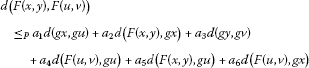
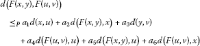
• (iv) there is some $h\in [0,1/2)$ such that for all $x,y,u,v\in X$ satisfying $gx\asymp gu$ and $gy\asymp gv$, there exists

  $${\mathrm{\Theta }}_{x,y,u,v}\in \{d(gx,gu),d(gy,gv),d(F(x,y),gu)\}$$

such that

$$d(F(x,y),F(u,v)){\le }_{P}h{\mathrm{\Theta }}_{x,y,u,v};$$

• (v) if $x_n\to x$ when $n\to \mathrm{\infty }$ in X, then $x_n\asymp x$ for n sufficiently large.

Then there exist $x,y\in X$ such that

$$F(x,y)=gx\mathit{\text{and}}F(y,x)=gy,$$

that is, F and g have a coupled coincidence point $(x,y)\in X\times X$.

Proof Since $F(X\times X)\subseteq g(X)$ (condition (i)), we can start from $x_0$, $y_0$ (condition (iii)) and construct sequences $\{g{x}_n\}$ and $\{g{y}_n\}$ in X such that

$$g{x}_n=F(x_{n-1},y_{n-1})\text{and}g{y}_n=F(y_{n-1},x_{n-1})$$

(3.11)

for all $n\in \mathbb{N}$. From (iii), we get $g{x}_0\asymp F(x_0,y_0)=g{x}_1$ and the condition (ii) implies that

$$g{x}_1=F(x_0,y_0)\asymp F(x_1,y_1)=g{x}_2.$$

By repeating this process, we have $g{x}_{n-1}\asymp g{x}_n$. Similarly, we can prove that $g{y}_{n-1}\asymp g{y}_n$ for all $n\in \mathbb{N}$.

Since $g{x}_{n-1}\asymp g{x}_n$ and $g{y}_{n-1}\asymp g{y}_n$ for all $n\in \mathbb{N}$, from (iv), we have that there exist $h\in [0,1/2)$ and

$$\begin{array}{rcl}{\mathrm{\Theta }}_1& \in & \{d(g{x}_{n-1},g{x}_n),d(g{y}_{n-1},g{y}_n),d(F(x_{n-1},y_{n-1}),g{x}_n)\}\\ =& \{d(g{x}_{n-1},g{x}_n),d(g{y}_{n-1},g{y}_n),0_E\}\end{array}$$

such that

$$d(g{x}_n,g{x}_{n+1})=d(F(x_{n-1},y_{n-1}),F(x_n,y_n)){\le }_{P}h{\mathrm{\Theta }}_1.$$

Similarly, one can show that there exists

$${\mathrm{\Theta }}_2\in \{d(g{x}_{n-1},g{x}_n),d(g{y}_{n-1},g{y}_n),0_E)\}$$

such that

$$d(g{y}_n,g{y}_{n+1})=d(F(y_{n-1},x_{n-1}),F(y_n,x_n)){\le }_{P}h{\mathrm{\Theta }}_2.$$

Now, denote ${\delta }_n=d(g{x}_n,g{x}_{n+1})+d(g{y}_n,g{y}_{n+1})$. Since the cases ${\mathrm{\Theta }}_1=0_E$ and ${\mathrm{\Theta }}_2=0_E$ are trivial, we have to consider the following four possibilities.

Case 1. $d(g{x}_n,g{x}_{n+1}){\le }_{P}hd(g{x}_{n-1},g{x}_n)$ and $d(g{y}_n,g{y}_{n+1}){\le }_{P}hd(g{y}_{n-1},g{y}_n)$. Adding up, we get that

$${\delta }_n{\le }_{P}h{\delta }_{n-1}{\le }_{P}2h{\delta }_{n-1}.$$

Case 2. $d(g{x}_n,g{x}_{n+1}){\le }_{P}hd(g{x}_{n-1},g{x}_n)$ and $d(g{y}_n,g{y}_{n+1}){\le }_{P}hd(g{x}_{n-1},g{x}_n)$. Then

$${\delta }_n{\le }_{P}2hd(g{x}_{n-1},g{x}_n){\le }_{P}2hd(g{x}_{n-1},g{x}_n)+2hd(g{y}_{n-1},g{y}_n)=2h{\delta }_{n-1}.$$

Case 3. $d(g{x}_n,g{x}_{n+1}){\le }_{P}hd(g{y}_{n-1},g{y}_n)$ and $d(g{y}_n,g{y}_{n+1}){\le }_{P}hd(g{x}_{n-1},g{x}_n)$. This case is treated analogously to Case 1.

Case 4. $d(g{x}_n,g{x}_{n+1}){\le }_{P}hd(g{y}_{n-1},g{y}_n)$ and $d(g{y}_n,g{y}_{n+1}){\le }_{P}hd(g{y}_{n-1},g{y}_n)$. This case is treated analogously to Case 2.

Thus, in all cases, we get ${\delta }_n{\le }_{P}2h{\delta }_{n-1}$ for all $n\in \mathbb{N}$, where $0\le 2h<1$. Therefore,

$${\delta }_n{\le }_{P}2h{\delta }_{n-1}{\le }_P{(2h)}^2{\delta }_{n-2}{\le }_P\cdots {\le }_P{(2h)}^n{\delta }_0,$$

and by the same argument as in Theorem 3.1, it is proved that $\{g{x}_n\}$ and $\{g{y}_n\}$ are Cauchy sequences in $g(X)$. By the completeness of $g(X)$, there exist $gx,gy\in g(X)$ such that $g{x}_n\to gx$ and $g{y}_n\to gy$.

From (v), we get $g{x}_n\asymp gx$ and $gy\asymp g{y}_n$ for all $n\ge 0$. Now, we prove that $F(x,y)=gx$ and $F(y,x)=gy$.

If $g{x}_n=gx$ and $g{y}_n=gy$ for some $n\ge 0$, from (iv) we have

$$\begin{array}{rcl}d(F(x,y),gx)& {\le }_P& d(F(x,y),g{x}_{n+1})+d(g{x}_{n+1},gx)\\ =& d(F(x,y),F(x_n,y_n))+d(g{x}_{n+1},gx)\\ {\le }_P& h{\mathrm{\Theta }}_{x,y,x_n,y_n}+d(g{x}_{n+1},gx),\end{array}$$

where ${\mathrm{\Theta }}_{x,y,x_n,y_n}\in \{d(gx,g{x}_n),d(gy,g{y}_n),d(F(x,y),g{x}_n)\}$. Let $c\in int(P)$ be fixed. If ${\mathrm{\Theta }}_{x,y,x_n,y_n}=d(gx,g{x}_n)=0_E$ or ${\mathrm{\Theta }}_{x,y,x_n,y_n}=d(gy,g{y}_n)=0_E$, then for n sufficiently large, we have that

$$d(F(x,y),gx)\ll c.$$

By property ($p_2$), it follows that $F(x,y)=gx$. If ${\mathrm{\Theta }}_{x,y,x_n,y_n}=d(F(x,y),g{x}_n)$, then we get that

$$\begin{array}{rcl}d(F(x,y),gx)& {\le }_P& hd(F(x,y),g{x}_n)+d(g{x}_{n+1},gx)\\ {\le }_P& hd(F(x,y),gx)+hd(gx,g{x}_n)+d(g{x}_{n+1},gx)\\ =& hd(F(x,y),gx)+d(g{x}_{n+1},gx).\end{array}$$

Now, it follows that for n sufficiently large,

$$\begin{array}{rcl}d(F(x,y),gx)& {\le }_P& \frac{1}{1-h}d(g{x}_{n+1},gx)\\ {\le }_P& \frac{1}{1-h}(1-h)c\\ =& c.\end{array}$$

Therefore, again by property ($p_2$), we get that $F(x,y)=gx$. Similarly, we can prove that $F(y,x)=gy$. Hence, $(x,y)$ is a coupled point of coincidence of F and g.

Then, we suppose that $(g{x}_n,g{y}_n)\ne (gx,gy)$ for all $n\ge 0$. For this, consider

$$\begin{array}{rcl}d(F(x,y),gx)& {\le }_P& d(F(x,y),g{x}_{n+1})+d(g{x}_{n+1},gx)\\ =& d(F(x,y),F(x_n,y_n))+d(g{x}_{n+1},gx)\\ {\le }_P& h{\mathrm{\Theta }}_{x,y,x_n,y_n}+d(g{x}_{n+1},gx),\end{array}$$

where ${\mathrm{\Theta }}_{x,y,x_n,y_n}\in \{d(gx,g{x}_n),d(gy,g{y}_n),d(F(x,y),g{x}_n)\}$. Let $c\in int(P)$ be fixed. If ${\mathrm{\Theta }}_{x,y,x_n,y_n}=d(gx,g{x}_n)$ or ${\mathrm{\Theta }}_{x,y,x_n,y_n}=d(gy,g{y}_n)$, then for n sufficiently large, we have that

$$d(F(x,y),gx)\ll h\cdot \frac{c}{2h}+\frac{c}{2}=c.$$

By property ($p_2$), it follows that $F(x,y)=gx$. If ${\mathrm{\Theta }}_{x,y,x_n,y_n}=d(F(x,y),g{x}_n)$, then we get that

$$\begin{array}{rcl}d(F(x,y),gx)& {\le }_P& hd(F(x,y),g{x}_n)+d(g{x}_{n+1},gx)\\ {\le }_P& hd(F(x,y),gx)+hd(gx,g{x}_n)+d(g{x}_{n+1},gx).\end{array}$$

Now, it follows that for n sufficiently large,

$$\begin{array}{rcl}d(F(x,y),gx)& {\le }_P& \frac{h}{1-h}d(gx,g{x}_n)+\frac{1}{1-h}d(g{x}_{n+1},gx)\\ \ll & \frac{h}{1-h}\cdot \frac{1-h}{h}\cdot \frac{c}{2}+\frac{1}{1-h}(1-h)\frac{c}{2}=c.\end{array}$$

Thus, again by property ($p_2$), we get that $F(x,y)=gx$.

Similarly, $F(y,x)=gy$ is obtained. Hence, $(x,y)$ is a coupled point of coincidence of the mappings F and g. □

Remark 3.6 It would be interesting to relate our Theorem 3.5 with Theorem 2.1 of Long et al. [39].

Putting $g=I_X$, where $I_X$ is the identity mapping from X into X in Theorem 3.5, we get the following corollary.

Corollary 3.7 Let $(X,d,⪯)$ be an ordered cone metric space over a solid cone P. Let $F:X\times X\to X$ be mappings. Suppose that the following hold:

• (i) X is complete;

• (ii) F satisfies property (2.4);

• (iii) there exist $x_0,y_0\in X$ such that $x_0\asymp F(x_0,y_0)$ and $y_0\asymp F(y_0,x_0)$;

• (iv) there is some $h\in [0,1/2)$ such that for all $x,y,u,v\in X$ satisfying $x\asymp u$ and $y\asymp v$, there exists

  $${\mathrm{\Theta }}_{x,y,u,v}\in \{d(x,u),d(y,v),d(F(x,y),u)\}$$

such that

$$d(F(x,y),F(u,v)){\le }_{P}h{\mathrm{\Theta }}_{x,y,u,v}.$$

• (v) if $x_n\to x$ when $n\to \mathrm{\infty }$ in X, then $x_n\asymp x$ for n sufficiently large.

Then there exist $x,y\in X$ such that

$$F(x,y)=x\mathit{\text{and}}F(y,x)=y,$$

that is, F has a coupled fixed point $(x,y)\in X\times X$.

4 Common coupled fixed point theorems lacking the mixed monotone property

Some questions arise naturally from Theorems 3.1 and 3.5. For example, one may ask if there are necessary conditions for the existence and uniqueness of a common coupled fixed point of F and g?

The next theorem provides a positive answer to this question with additional hypotheses to Theorems 3.1 and 3.5.

For the given partial order ⪯ on the set X, we will denote also by ⪯ the order on $X\times X$ given by

$$(x_1,y_1)⪯(x_2,y_2)⟺x_1⪯x_2\text{and}{y}_1⪰y_2.$$

(4.1)

Theorem 4.1 In addition to the hypotheses of Theorem  3.1, suppose that for every $(x,y),(x^{\ast },y^{\ast })\in X\times X$, there exists $(u,v)\in X\times X$ such that

$$(F(u,v),F(v,u))\asymp (F(x,y),F(y,x))$$

and

$$(F(u,v),F(v,u))\asymp (F(x^{\ast },y^{\ast }),F(y^{\ast },x^{\ast })).$$

If F and g are $w^{\ast }$-compatible, then F and g have a unique common coupled fixed point, that is, there exists a unique $(\hat{u},\hat{v})\in X\times X$ such that

$$\hat{u}=g\hat{u}=F(\hat{u},\hat{v})\mathit{\text{and}}\hat{v}=g\hat{v}=F(\hat{v},\hat{u}).$$

Proof From Theorem 3.1, the set of coupled coincidence points of F and g is nonempty. Suppose $(x,y)$ and $(x^{\ast },y^{\ast })$ are coupled coincidence points of F, that is, $gx=F(x,y)$, $gy=F(y,x)$, $g{x}^{\ast }=F(x^{\ast },y^{\ast })$ and $g{y}^{\ast }=F(y^{\ast },x^{\ast })$. We will prove that

$$gx=g{x}^{\ast }\text{and}gy=g{y}^{\ast }.$$

(4.2)

By assumption, there exists $(u,v)\in X\times X$ such that

$$(F(u,v),F(v,u))\asymp (F(x,y),F(y,x))$$

and

$$(F(u,v),F(v,u))\asymp (F(x^{\ast },y^{\ast }),F(y^{\ast },x^{\ast })).$$

Put $u_0=u$, $v_0=v$ and choose $u_1,v_1\in X$ so that $g{u}_1=F(u_0,v_0)$ and $g{v}_1=F(v_0,u_0)$. Then, similarly as in the proof of Theorem 3.1, we can inductively define sequences $\{g{u}_n\}$, $\{g{v}_n\}$ with

$$g{u}_{n+1}=F(u_n,v_n)\text{and}g{v}_{n+1}=F(v_n,u_n)$$

for all n. Further, set $x_0=x$, $y_0=y$, $x_0^{\ast }=x^{\ast }$, $y_0^{\ast }=y^{\ast }$ and, in a similar way, define the sequences $\{g{x}_n\}$, $\{g{y}_n\}$ and $\{g{x}_n^{\ast }\}$, $\{g{y}_n^{\ast }\}$. Then it is easy to show that

$$g{x}_n\to F(x,y),g{y}_n\to F(y,x)$$

and

$$g{x}_n^{\ast }\to F(x^{\ast },y^{\ast }),g{y}_n^{\ast }\to F(y^{\ast },x^{\ast })$$

as $n\to \mathrm{\infty }$.

Since

$$(gx,gy)=(g{x}_1,g{y}_1)=(F(x,y),F(y,x))\asymp (F(u,v),F(v,u))=(g{u}_1,g{v}_1),$$

we have $gx\asymp g{u}_1$ and $gy\asymp g{v}_1$. It is easy to show that, similarly,

$$(gx,gy)\asymp (g{u}_n,g{v}_n)$$

for all $n\ge 1$, that is, $gx\asymp g{u}_n$ and $gy\asymp g{v}_n$ for all $n\ge 1$. Thus, from (3.1), we have

$$\begin{array}{rcl}d(g{u}_{n+1},gx)& =& d(F(u_n,v_n),F(x,y))\\ {\le }_P& a_{1}d(g{u}_n,gx)+a_{2}d(F(u_n,v_n),g{u}_n)+a_{3}d(g{v}_n,gy)\\ +a_{4}d(F(x,y),gx)+a_{5}d(F(u_n,v_n),gx)+a_{6}d(F(x,y),g{u}_n)\\ =& a_{1}d(g{u}_n,gx)+a_{2}d(g{u}_{n+1},g{u}_n)+a_{3}d(g{v}_n,gy)\\ +a_{4}d(gx,gx)+a_{5}d(g{u}_{n+1},gx)+a_{6}d(gx,g{u}_n)\\ {\le }_P& a_{1}d(g{u}_n,gx)+a_2[d(g{u}_{n+1},gx)+d(gx,g{u}_n)]+a_{3}d(g{v}_n,gy)\\ +a_{5}d(g{u}_{n+1},gx)+a_{6}d(gx,g{u}_n),\end{array}$$

that is,

$$(1-a_2-a_5)d(g{u}_{n+1},gx){\le }_P(a_1+a_2+a_6)d(g{u}_n,gx)+a_{3}d(g{v}_n,gy).$$

In the same way, starting from $d(g{v}_{n+1},gy)$, we can show that

$$(1-a_2-a_5)d(g{v}_{n+1},gy){\le }_P(a_1+a_2+a_6)d(g{v}_n,gy)+a_{3}d(g{u}_n,gx).$$

Thus,

(4.3)

In a similar way, starting from $d(gx,g{u}_{n+1})$, resp. $d(gy,g{v}_{n+1})$, and adding up the obtained inequalities, one gets that

(4.4)

Finally, adding up (4.3) and (4.4), we obtain that

$$d(g{u}_{n+1},gx)+d(g{v}_{n+1},gy){\le }_P\lambda [d(g{u}_n,gx)+d(g{v}_n,gy)],$$

(4.5)

where λ is determined as in (3.8), and hence $0\le \lambda <1$.

By inequality (4.5) n time, we have

It follows from ${\lambda }^n[d(g{u}_0,gx)+d(g{v}_0,gy)]\to 0_E$ as $n\to \mathrm{\infty }$ that

$$d(g{u}_n,gx)+d(g{v}_n,gy)\ll c$$

for all $c\in int(P)$ and large n. Since

$$0_E{\le }_{P}d(g{u}_n,gx){\le }_{P}d(g{u}_n,gx)+d(g{v}_n,gy),$$

it follows by ($p_3$) that $d(g{u}_n,gx)\ll c$ for large n, and so $g{u}_n\to gx$ when $n\to \mathrm{\infty }$. Similarly, $g{v}_n\to gy$ when $n\to \mathrm{\infty }$. By the same procedure, one can show that $g{u}_n\to g{x}^{\ast }$ and $g{v}_n\to g{y}^{\ast }$ as $n\to \mathrm{\infty }$. By the uniqueness of the limit, we get $gx=g{x}^{\ast }$ and $gy=g{y}^{\ast }$, i.e., (4.2) is proved. Therefore, $(gx,gy)$ is the unique coupled point of coincidence of F and g.

Note that if $(gx,gy)$ is a coupled point of coincidence of F and g, then $(gy,gx)$ is also a coupled point of coincidence of F and g. Then $gx=gy$ and therefore $(gx,gx)$ is the unique coupled point of coincidence of F and g.

Next, we show that F and g have a common coupled fixed point. Let $\hat{u}:=gx$. Then we have $\hat{u}=gx=F(x,x)$. Since F and g are $w^{\ast }$-compatible, we have

$$g\hat{u}=ggx=gF(x,x)=F(gx,gx)=F(\hat{u},\hat{u}).$$

Thus, $(g\hat{u},g\hat{u})$ is a coupled point of coincidence of F and g. By the uniqueness of a coupled point of coincidence of F and g, we get $g\hat{u}=gx$. Therefore, $\hat{u}=g\hat{u}=F(\hat{u},\hat{u})$, that is, $(\hat{u},\hat{u})$ is a common coupled fixed point of F and g.

Finally, we show the uniqueness of a common coupled fixed point of F and g. Let $(\tilde{u},\tilde{u})\in X\times X$ be another common coupled fixed point of F and g. So,

$$\tilde{u}=g\tilde{u}=F(\tilde{u},\tilde{u}).$$

Then $(g\hat{u},g\hat{u})$ and $(g\tilde{u},g\tilde{u})$ are two common coupled points of coincidence of F and g and, as was previously proved, it must be $g\hat{u}=g\tilde{u}$, and so $\hat{u}=g\hat{u}=g\tilde{u}=\tilde{u}$. This completes the proof. □

Next, we give some illustrative example which supports Theorem 4.1, while the results of Nashine et al. [33] do not.

Example 4.2 Let $X=\mathbb{R}$ be ordered by the following relation:

$$x⪯y⟺x\ge y.$$

Let $E=C_{\mathbb{R}}^1[0,1]$ with $\parallel f\parallel ={\parallel f\parallel }_{\mathrm{\infty }}+{\parallel f^{\mathrm{\prime }}\parallel }_{\mathrm{\infty }}$ for all $f\in E$ and

$$P=\{f\in E:f(t)\ge 0\text{ for }t\in [0,1]\}.$$

It is well known (see, e.g., [40]) that the cone P is not normal. Let

$$d(x,y)=|x-y|\phi$$

for all $x,y\in X$, for a fixed $\phi \in P$ (e.g., $\phi (t)=e^t$ for $t\in [0,1]$). Then $(X,d)$ is a complete ordered cone metric space over a non-normal solid cone.

Let $g:X\to X$ and $F:X\times X\to X$ be defined by

$$gx=\frac{x^2}{2}\text{and}F(x,y)=\frac{x^2+y^2}{8}.$$

Consider $y_1=2$ and $y_2=1$, we have for $x=3$, we get $y_1=2⪯1=y_2$, but

$$F(x,y_1)=\frac{13}{8}⪯\frac{10}{8}=F(x,y_2).$$

So, the mapping F does not satisfy the mixed g-monotone property. Therefore, Theorems 3.1 and 3.2 of Nashine et al. [33] cannot be used to reach this conclusion.

Now, we show that Theorem 4.1 can be used for this case.

Take $a_1=a_3=\frac{1}{4}$ and $a_2=a_4=a_5=a_6=0$. We will check that the condition (3.1) in Theorem 3.1 holds.

For $x,y,u,v\in X$ satisfying $gu\asymp gx$ and $gv\asymp gy$, we have

$$\begin{array}{rcl}d(F(x,y),F(u,v))& =& |\frac{x^2+y^2}{8}-\frac{u^2+v^2}{8}|\phi \\ {\le }_P& \frac{1}{4}|\frac{x^2}{2}-\frac{u^2}{2}|\phi +\frac{1}{4}|\frac{y^2}{2}-\frac{v^2}{2}|\phi \\ =& \frac{1}{4}d(gx,gu)+\frac{1}{4}d(gy,gv)\\ =& a_{1}d(gx,gu)+a_{3}d(gy,gv).\end{array}$$

Next, we show that F and g are $w^{\ast }$-compatible. We note that if $gx=F(x,x)$, then we get only one case, that is, $x=0$, and hence

$$gF(x,x)=gF(0,0)=g0=0=F(0,0)=F(g0,g0)=F(gx,gx).$$

Therefore, F and g are $w^{\ast }$-compatible.

Moreover, other conditions in Theorem 4.1 are also satisfied. Now, we can apply Theorem 4.1 to conclude the existence of a unique common coupled fixed point of F and g that is a point $(0,0)$.

The following uniqueness result corresponding to Theorem 3.5 can be proved in the same way as Theorem 4.1.

Theorem 4.3 In addition to the hypotheses of Theorem  3.5, suppose that for every $(x,y),(x^{\ast },y^{\ast })\in X\times X$, there exists $(u,v)\in X\times X$ such that

$$(F(u,v),F(v,u))\asymp (F(x,y),F(y,x))$$

and

$$(F(u,v),F(v,u))\asymp (F(x^{\ast },y^{\ast }),F(y^{\ast },x^{\ast })).$$

If F and g are $w^{\ast }$-compatible, then F and g have a unique coupled common fixed point, that is, there exists a unique $(\hat{u},\hat{v})\in X\times X$ such that

$$\hat{u}=g\hat{u}=F(\hat{u},\hat{v})\mathit{\text{and}}\hat{v}=g\hat{v}=F(\hat{v},\hat{u}).$$

References

Turinici M: Abstract comparison principles and multivariable Gronwall-Bellman inequalities. J. Math. Anal. Appl. 1986, 117: 100–127. 10.1016/0022-247X(86)90251-9
Ran ACM, Reurings MCB: A fixed point theorem in partially ordered sets and some applications to matrix equations. Proc. Am. Math. Soc. 2004, 132(5):1435–1443. 10.1090/S0002-9939-03-07220-4
Altun I, Damjanović B, Djorić D: Fixed point and common fixed point theorems on ordered cone metric spaces. Appl. Math. Lett. 2009, 23: 310–316.
Aydi H, Nashine HK, Samet B, Yazidi H: Coincidence and common fixed point results in partially ordered cone metric spaces and applications to integral equations. Nonlinear Anal. 2011, 74: 6814–6825. 10.1016/j.na.2011.07.006
Kadelburg Z, Pavlović M, Radenović S: Common fixed point theorems for ordered contractions and quasicontractions in ordered cone metric spaces. Comput. Math. Appl. 2010, 59: 3148–3159. 10.1016/j.camwa.2010.02.039
Nieto JJ, López RR: Contractive mapping theorems in partially ordered sets and applications to ordinary differential equations. Order 2005, 22: 223–239. 10.1007/s11083-005-9018-5
Guo D, Lakshmikantham V: Coupled fixed points of nonlinear operators with applications. Nonlinear Anal., Theory Methods Appl. 1987, 11: 623–632. 10.1016/0362-546X(87)90077-0
Bhaskar TG, Lakshmikantham V: Fixed point theorems in partially ordered metric spaces and applications. Nonlinear Anal. 2006, 65: 1379–1393. 10.1016/j.na.2005.10.017
Harjani J, López B, Sadarangani K: Fixed point theorems for mixed monotone operators and applications to integral equations. Nonlinear Anal. 2011, 74: 1749–1760. 10.1016/j.na.2010.10.047
Luong NV, Thuan NX: Coupled fixed points in partially ordered metric spaces and application. Nonlinear Anal. 2011, 74: 983–992. 10.1016/j.na.2010.09.055
Luong NV, Thuan NX: Coupled fixed point theorems for mixed monotone mappings and an application to integral equations. Comput. Math. Appl. 2011. doi:10.1016/j.camwa.2011.10.011
Caballero J, Harjani J, Sadarangani K: Positive solutions for a class of singular fractional boundary value problems. Comput. Math. Appl. 2011, 62(3):1325–1332. 10.1016/j.camwa.2011.04.013
Jleli M, Samet B: On positive solutions for a class of singular nonlinear fractional differential equations. Bound. Value Probl. 2012., 2012: Article ID 73
Lakshmikantham V, Ćirić LB: Coupled fixed point theorems for nonlinear contractions in partially ordered metric spaces. Nonlinear Anal. 2009, 70: 4341–4349. 10.1016/j.na.2008.09.020
Abbas M, Sintunavarat W, Kumam P: Coupled fixed point of generalized contractive mappings on partially ordered G -metric spaces. Fixed Point Theory Appl. 2012., 2012: Article ID 31
Choudhury BS, Kundu A: A coupled coincidence point result in partially ordered metric spaces for compatible mappings. Nonlinear Anal. 2010, 73: 2524–2531. 10.1016/j.na.2010.06.025
Nashine HK, Shatanawi W: Coupled common fixed point theorems for pair of commuting mappings in partially ordered complete metric spaces. Comput. Math. Appl. 2011, 62: 1984–1993. 10.1016/j.camwa.2011.06.042
Samet B: Coupled fixed point theorems for a generalized Meir-Keeler contraction in partially ordered metric spaces. Nonlinear Anal. 2010, 72: 4508–4517. 10.1016/j.na.2010.02.026
Karapınar E, Kumam P, Sintunavarat W: Coupled fixed point theorems in cone metric spaces with a c -distance and applications. Fixed Point Theory Appl. 2012., 2012: Article ID 194
Aydi H, Karapınar E, Shatanawi W: Coupled coincidence points in ordered cone metric spaces with c -distance. J. Appl. Math. 2012., 2012: Article ID 312078
Aydi H, Karapınar E, Shatanawi W:Coupled fixed point results for -weakly contractive condition in ordered partial metric spaces. Comput. Math. Appl. 2011, 62(12):4449–4460. 10.1016/j.camwa.2011.10.021
Ding H-S, Karapınar E: A note on some coupled fixed point theorems on G -metric space. J. Inequal. Appl. 2012., 2012: Article ID 170
Hung NM, Karapınar E, Luong NV: Coupled coincidence point theorem in partially ordered metric spaces via implicit relation. Abstr. Appl. Anal. 2012., 2012: Article ID 796964
Karapınar E, Türkoǧlu AD: Best approximations theorem for a couple in cone Banach spaces. Fixed Point Theory Appl. 2010., 2010: Article ID 784578
Karapınar E, Kaymakcalan B, Tas K: On coupled fixed point theorems on partially ordered G -metric spaces. J. Inequal. Appl. 2012., 2012: Article ID 200
Sintunavarat W, Cho YJ, Kumam P: Coupled coincidence point theorems for contractions without commutative condition in intuitionistic fuzzy normed spaces. Fixed Point Theory Appl. 2011., 2011: Article ID 81
Sintunavarat W, Cho YJ, Kumam P: Coupled fixed point theorems for weak contraction mapping under F -invariant set. Abstr. Appl. Anal. 2012., 2012: Article ID 324874
Sintunavarat W, Cho YJ, Kumam P: Coupled fixed-point theorems for contraction mapping induced by cone ball-metric in partially ordered spaces. Fixed Point Theory Appl. 2012., 2012: Article ID 128
Sintunavarat W, Petruşel A, Kumam P:Common coupled fixed point theorems for -compatible mappings without mixed monotone property. Rend. Circ. Mat. Palermo 2012, 61: 361–383. doi:10.1007/s12215–012–0096–0 10.1007/s12215-012-0096-0
Sintunavarat W, Kumam P, Cho YJ: Coupled fixed point theorems for nonlinear contractions without mixed monotone property. Fixed Point Theory Appl. 2012., 2012: Article ID 170
Huang LG, Zhang X: Cone metric spaces and fixed point theorems of contractive mappings. J. Math. Anal. Appl. 2007, 332: 1468–1476. 10.1016/j.jmaa.2005.03.087
Janković S, Kadelburg Z, Radenović S: On cone metric spaces: a survey. Nonlinear Anal. 2011, 74: 2591–2601. 10.1016/j.na.2010.12.014
Nashine HK, Kadelburg Z, Radenović S:Coupled common fixed point theorems for -compatible mappings in ordered cone metric spaces. Appl. Math. Comput. 2012, 218: 5422–5432. 10.1016/j.amc.2011.11.029
Karapınar E: Couple fixed point theorems for nonlinear contractions in cone metric spaces. Comput. Math. Appl. 2010, 59: 3656–3668. 10.1016/j.camwa.2010.03.062
Shatanawi W: Partially ordered cone metric spaces and coupled fixed point results. Comput. Math. Appl. 2010, 60: 2508–2515. 10.1016/j.camwa.2010.08.074
Abbas M, Khan MA, Radenović S: Common coupled fixed point theorem in cone metric space for w -compatible mappings. Appl. Math. Comput. 2010, 217: 195–202. 10.1016/j.amc.2010.05.042
Ðorić D, Kadelburg Z, Radenović S: Coupled fixed point results for mappings without mixed monotone property. Appl. Math. Lett. 2012. doi:10.1016/j.aml.2012.02.022
Rezapour S, Hamlbarani R: Some notes on paper ‘Cone metric spaces and fixed point theorems of contractive mappings’. J. Math. Anal. Appl. 2008, 345: 719–724. 10.1016/j.jmaa.2008.04.049
Long W, Rhoades BE, Rajovic M: Coupled coincidence points for two mappings in metric spaces and cone metric spaces. Fixed Point Theory Appl. 2012., 2012: Article ID 66
Vandergraft JS: Newton method for convex operators in partially ordered spaces. SIAM J. Numer. Anal. 1967, 4(3):406–432. 10.1137/0704037
Acknowledgements
The authors would like to thank Professor Hichem Ben-El-Mechaiekh and the referee for valuable comments. The second author would like to thank the Research Professional Development Project under the Science Achievement Scholarship of Thailand (SAST) and the third author would like to thank the Commission on Higher Education, the Thailand Research Fund and KMUTT under Grant No. MRG5580213 for financial support during the preparation of this manuscript.
Author information
Authors and Affiliations
Corresponding authors
Additional information
Competing interests
The authors declare that they have no competing interests.
Authors’ contributions
All authors contributed equally and significantly in writing this paper. All authors read and approved the final manuscript.
Rights and permissions
Open Access This article is distributed under the terms of the Creative Commons Attribution 2.0 International License ( https://creativecommons.org/licenses/by/2.0 ), which permits unrestricted use, distribution, and reproduction in any medium, provided the original work is properly cited.
About this article
Cite this article
Agarwal, R.P., Sintunavarat, W. & Kumam, P. Coupled coincidence point and common coupled fixed point theorems lacking the mixed monotone property. Fixed Point Theory Appl 2013, 22 (2013). https://doi.org/10.1186/1687-1812-2013-22
Received:
Accepted:
Published:
DOI: https://doi.org/10.1186/1687-1812-2013-22